PINN Fluid Analysis
Overview
Professor! Today we're talking about PINN fluid analysis, right? What is it about?
Theoretical Foundations of PINNs for Fluids
The Basic Structure of a PINN
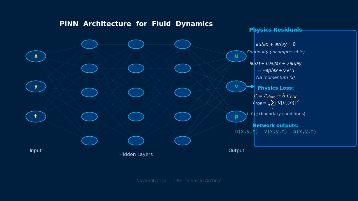
A physics-informed neural network represents the flow field \( (\mathbf{u}, p) \) with a neural network \( \mathcal{N}(\mathbf{x}, t; \theta) \) and trains it by embedding the governing-equation residual in the loss function. Derivatives are taken exactly by automatic differentiation, so no mesh is required. The loss is typically a weighted sum of three terms:
$$ \mathcal{L}(\theta) = \lambda_{pde}\,\mathcal{L}_{PDE} + \lambda_{bc}\,\mathcal{L}_{BC/IC} + \lambda_{data}\,\mathcal{L}_{data} $$
\( \mathcal{L}_{PDE} \) is the Navier-Stokes residual at collocation points (momentum plus continuity), \( \mathcal{L}_{BC/IC} \) the boundary and initial condition residual, and \( \mathcal{L}_{data} \) the mismatch against measurements. That third term is what matters most: it lets data and physical law be satisfied on the same footing, which is the PINN's distinguishing feature.
Formulation Choices Specific to Fluids
| Option | What it does | Character |
|---|---|---|
| Velocity-pressure form | Output \( (u, v, w, p) \) directly | Straightforward, but continuity must be satisfied through the loss (soft constraint) |
| Stream-function form (2-D) | Output \( \psi \), set \( u = \psi_y, v = -\psi_x \) | Satisfies continuity exactly by construction — strong choice for 2-D incompressible flow |
| Nondimensionalization | Solve the Re-scaled equations | Effectively mandatory; dimensional variables wreck the loss scaling |
Know the Map of Strengths and Weaknesses First
PINNs don't need a mesh, right? Doesn't that make CFD solvers obsolete?
Let's be clear-eyed about this. For pure forward problems — given geometry and boundary conditions, find the flow — a mature finite-volume solver is orders of magnitude faster and more accurate. That's a result the research community broadly agrees on. Where PINNs earn their place is elsewhere: ① inverse problems (infer viscosity, inflow profile, or boundary geometry from observations), ② data assimilation (reconstruct a physically consistent full field from sparse PIV or sensor data), ③ recovering quantities you cannot measure from ones you can — pressure fields being the classic case. So use them not as a CFD replacement but as an estimator that couples data with physics.
Numerical Methods That Make Training Work
Loss Balancing Is the Hardest Part
PDE, boundary, and data residuals differ by orders of magnitude, and with fixed weights one term dominates and training fails. The practical escalation:
- Nondimensionalize thoroughly — bring every term to O(1). This alone often solves it
- Hard boundary conditions — transform the output with a distance function so BCs hold exactly, eliminating \( \mathcal{L}_{BC} \) entirely (a large convergence improvement)
- Automatic weighting — update \( \lambda \) from gradient-norm ratios (GradNorm family), NTK-theoretic weighting, or residual-based adaptive weights
Collocation Points and Network Design
Sample collocation points uniformly at random (or by Latin hypercube), then add points adaptively where the residual is large. Seed steep-gradient regions — boundary layers, separation points — densely from the start. An MLP with tanh activations is standard; for high-wavenumber flow structures, Fourier feature embedding (lifting inputs through trigonometric functions) is the standard remedy for spectral bias, the tendency of networks to learn low frequencies first. For optimization, "Adam to get globally down, then L-BFGS to polish" is empirically the most reliable.
The High-Reynolds-Number Wall
As Re rises, the flow develops fine structure and strong nonlinearity, and a single-network PINN degrades quickly. Resolving turbulence in a DNS sense is outside the PINN's range; the practical ceiling is laminar to transitional flow, on the order of Re in the hundreds to low thousands. The countermeasures used in research and practice are: ① domain decomposition (XPINN and relatives: split space into subdomains joined at interfaces), ② causality-respecting training (weight early times first so the network cannot cheat by fitting late times), ③ combining with RANS so the target is the mean field.
Applying It in Practice
The Winning Pattern — Field Reconstruction from Observations
The signature success of PINNs in fluids is turning sparse, noisy measurements into a physically consistent full field:
- PIV/PTV plus PINN — from sparse in-plane velocity measurements, recover both the velocity field satisfying continuity and momentum, and the pressure field you could not measure
- Flow estimation from a few sensors — interpolate interior fields from wall pressures or flow rates, more physically defensible than pure interpolation
- Parameter inference — treat effective viscosity, inflow profile, or heat transfer coefficient as unknowns optimized jointly with the observations
Standard Workflow
- Nondimensionalize — organize around Re with characteristic length and velocity; bring all variables to O(1)
- Choose the formulation — stream function first for 2-D incompressible; make boundary conditions hard wherever possible
- Training setup — MLP (4–8 layers, 64–128 units) plus Fourier features; Adam then L-BFGS
- Convergence diagnosis — do not watch the loss value alone; visualize the spatial distribution of the PDE residual (concentration means you need adaptive sampling)
- Validation — quantitative comparison against a reference CFD solution, conservation quantities (does the mass flow balance across sections?), and held-out observation points
Verify with the Same Discipline as Conventional V&V
Reporting a PINN result deserves the same rigor as a CFD result. A falling loss does not mean the problem is solved. At minimum, report: ① norm-wise error against an independent reference (CFD or analytic), ② conservation checks (mass flow equality between sections), ③ prediction error at held-out observation points, ④ stability of results across random seeds and re-sampled collocation points. A small residual loss can coexist with a large global error — residual and error are different quantities, exactly as in classical numerical analysis.
Frameworks and Implementation
Framework Comparison
| Framework | Character | Best for |
|---|---|---|
| DeepXDE | The reference general-purpose PINN library; geometry, BCs, adaptive sampling built in | Research and prototyping broadly |
| NVIDIA PhysicsNeMo (formerly Modulus) | Large-scale, multi-GPU, industrial focus; imports STL geometry | Industrial-scale training |
| PyTorch / JAX from scratch | Maximum freedom for custom weighting and formulations | Method development |
| NeuralPDE.jl (Julia) | Integrated with the SciML ecosystem | Julia-based research |
DeepXDE Skeleton (2-D Cavity Flow)
import deepxde as dde

def ns_residual(x, y):            # y = (u, v, p)
    u, v, p = y[:, 0:1], y[:, 1:2], y[:, 2:3]
    u_x = dde.grad.jacobian(y, x, i=0, j=0); u_y = dde.grad.jacobian(y, x, i=0, j=1)
    # ... take each derivative by automatic differentiation and return the three
    #     nondimensional NS residuals (two momentum + continuity)

geom = dde.geometry.Rectangle([0, 0], [1, 1])
bc = [dde.icbc.DirichletBC(geom, lid_u, on_lid, component=0), ...]
data = dde.data.PDE(geom, ns_residual, bc, num_domain=5000, num_boundary=400)
net = dde.nn.FNN([2] + [64] * 6 + [3], "tanh", "Glorot normal")
model = dde.Model(data, net)
model.compile("adam", lr=1e-3); model.train(iterations=20000)
model.compile("L-BFGS"); model.train()   # polish
In practice you add nondimensionalization, hard BCs, loss weighting, and residual visualization on top of this skeleton. Always archive the training history (each loss component over iterations) and attach it to the report.
Research Frontiers
Choosing Between PINNs and Operator Learning
Where a PINN solves one problem with one network, FNO (Fourier Neural Operator) and DeepONet learn the mapping itself — boundary conditions or geometry to solution — from large sets of CFD results. Once trained, inference on a new condition takes milliseconds, so for many-case evaluation (optimization, real-time prediction) operator learning wins. Conversely, for inverse problems and assimilation where you have only one case's worth of data, the PINN wins. "Repeated evaluation → operator learning; data fusion → PINN" is the division of labor that has settled in. Physics-informed operator learning (PINO) combines both and is active.
Theory of Why They Fail
Recent years brought theory explaining PINN training failures. Neural tangent kernel analysis quantifies the imbalance in convergence rates between loss terms, underpinning automatic weighting schemes. Spectral bias explains why boundary layers and high-wavenumber structure resist learning; causality violation explains why minimizing residuals at late times first breaks time-evolution problems (the motivation for causal training). Yesterday's heuristics now have principled justifications.
Hybrids with Differentiable Solvers
Making a conventional solver itself automatically differentiable (differentiable CFD) and using networks only for turbulence closure terms is the hybrid line gaining practical ground. Numerical robustness and conservation stay with the solver while the network learns only the modeling error, sidestepping the pure PINN's weaknesses in conservation and high Re. Learned corrections to RANS closures and learned SGS models for LES are the closest to industrial deployment.
Troubleshooting
Symptoms, Causes, and Fixes
| Symptom | Likely cause | Fix |
|---|---|---|
| Loss falls but the field collapses to zero/uniform | Converged to the trivial solution (u=0 minimizes the residual when the BC term is weak) | Hard boundary conditions; raise \( \lambda_{bc} \); add data points |
| Only the pressure field is badly off | Pressure indeterminacy (no reference); only its gradient appears in the equations | Pin pressure at one point; compare against reference with the mean removed |
| Boundary layers and separation come out blurred | Spectral bias; too few collocation points | Fourier features; densify near walls; adaptive sampling |
| Training collapses suddenly at higher Re | Nonlinearity and fine structure exceed network capacity and the optimizer | Re-check nondimensionalization; domain decomposition (XPINN); continuation from a lower-Re solution |
| Unsteady runs disagree at late times | Causality violation (all times trained at once) | Causal training; time-marching in segments |
| Diverges during the L-BFGS stage | Adam stage not converged enough; ill-conditioned loss | Extend Adam; revisit weight balance; restart at lower learning rate |
| Inferred parameters differ every run | Non-uniqueness from insufficient observational information | Add and optimize sensor placement; add priors (regularization); report confidence intervals |
A Three-Question Adoption Test
So how do I decide whether PINNs are right for my project?
Three questions settle it. Q1: Do you want to fuse measurements with physical law? If yes, it's a candidate; if no — a pure forward problem — use conventional CFD, full stop. Q2: Is the target laminar-to-transitional, or a mean field? Instantaneous turbulent fields are out of reach. Q3: Can you produce a means of validation — a reference solution or held-out observations? If not, you cannot demonstrate credibility, so don't start. Three yeses, and the low-risk entry is to start small with a proven pattern such as PIV pressure recovery or parameter identification.
Related: PINNs for structural analysis, all PINN articles, Kriging surrogates (as a data-driven contrast).
detail
error