Magnetic Vector Potential
Magnetic Vector Potential: Theoretical Foundations
Vector Potential$\mathbf{A}$
Professor, what is the magnetic vector potential?
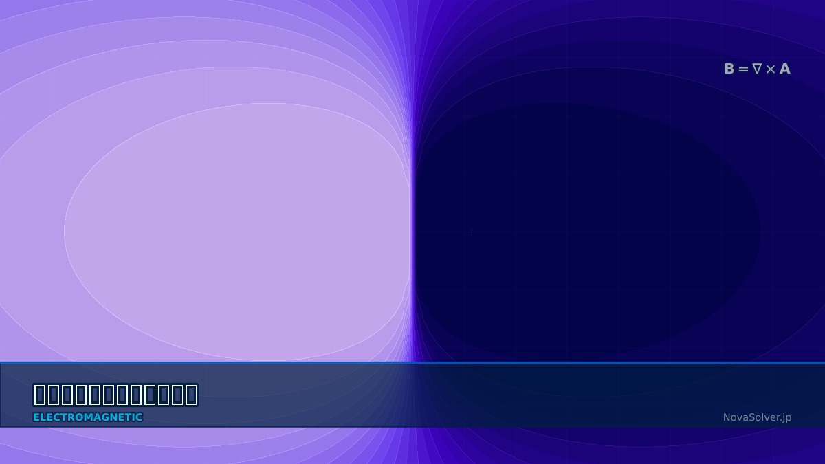
The "potential" for magnetic flux density $\mathbf{B}$. Since $\mathbf{B}$ has zero divergence ($\nabla \cdot \mathbf{B} = 0$), it can always be expressed as the curl of some vector field $\mathbf{A}$:
$$ \mathbf{B} = \nabla \times \mathbf{A} $$
It corresponds to the electric potential $\phi$ in electrostatic fields.
Correspondence:
Electrostatic Field Magnetostatic Field $\mathbf{E} = -\nabla\phi$ $\mathbf{B} = \nabla \times \mathbf{A}$ $\phi$: Scalar $\mathbf{A}$: Vector (3 components) Poisson: $\nabla^2\phi = -\rho/\varepsilon$ $\nabla^2\mathbf{A} = -\mu\mathbf{J}$ (Coulomb gauge)
Gauge Condition
$\mathbf{A}$ is not uniquely determined (adding the gradient of any scalar field $\psi$ does not change $\mathbf{B}$). To ensure uniqueness, impose a gauge condition:
- Coulomb Gauge: $\nabla \cdot \mathbf{A} = 0$ — Standard for magnetostatics
- Lorenz Gauge: $\nabla \cdot \mathbf{A} + \mu\varepsilon \partial\phi/\partial t = 0$ — For dynamic problems
2D $A_z$
In 2D problems (uniform in the $z$ direction), $\mathbf{A} = A_z(x,y) \hat{z}$ becomes a scalar problem. Magnetic field lines are contours of $A_z$. This is the greatest advantage of 2D magnetic field FEM.
Summary
- $\mathbf{B} = \nabla \times \mathbf{A}$ — The basis of magnetic field FEM
- Uniqueness guaranteed by gauge condition — Coulomb gauge is standard
- Scalar problem for $A_z$ in 2D — Magnetic field lines = $A_z$ contours
Coffee Break Trivia Corner
Magnetic Vector Potential—Why a "Quantity Without Physical Substance" Supports FEM
The magnetic vector potential A (B=rot A) is sometimes called a "shadow quantity" of electric and magnetic fields; it cannot be measured directly but is indispensable for computation. The reason FEM magnetic field analysis uses A, not B, as the unknown is because automatically satisfying div B=0 (magnetic flux continuity) is more important than numerically handling rot B=μ₀J. In the A formulation, div B=0 is automatically guaranteed as rot(rot A)=0. In the 1970s, Oliver C. Zienkiewicz and others applied the A formulation to FEM, and it now forms the foundation of all major magnetic field FEM solvers.
Professor, what is the magnetic vector potential?
The "potential" for magnetic flux density $\mathbf{B}$. Since $\mathbf{B}$ has zero divergence ($\nabla \cdot \mathbf{B} = 0$), it can always be expressed as the curl of some vector field $\mathbf{A}$:
It corresponds to the electric potential $\phi$ in electrostatic fields.
Correspondence:
| Electrostatic Field | Magnetostatic Field |
|---|---|
| $\mathbf{E} = -\nabla\phi$ | $\mathbf{B} = \nabla \times \mathbf{A}$ |
| $\phi$: Scalar | $\mathbf{A}$: Vector (3 components) |
| Poisson: $\nabla^2\phi = -\rho/\varepsilon$ | $\nabla^2\mathbf{A} = -\mu\mathbf{J}$ (Coulomb gauge) |
$\mathbf{A}$ is not uniquely determined (adding the gradient of any scalar field $\psi$ does not change $\mathbf{B}$). To ensure uniqueness, impose a gauge condition:
- Coulomb Gauge: $\nabla \cdot \mathbf{A} = 0$ — Standard for magnetostatics
- Lorenz Gauge: $\nabla \cdot \mathbf{A} + \mu\varepsilon \partial\phi/\partial t = 0$ — For dynamic problems
2D $A_z$
In 2D problems (uniform in the $z$ direction), $\mathbf{A} = A_z(x,y) \hat{z}$ becomes a scalar problem. Magnetic field lines are contours of $A_z$. This is the greatest advantage of 2D magnetic field FEM.
Summary
- $\mathbf{B} = \nabla \times \mathbf{A}$ — The basis of magnetic field FEM
- Uniqueness guaranteed by gauge condition — Coulomb gauge is standard
- Scalar problem for $A_z$ in 2D — Magnetic field lines = $A_z$ contours
Magnetic Vector Potential—Why a "Quantity Without Physical Substance" Supports FEM
The magnetic vector potential A (B=rot A) is sometimes called a "shadow quantity" of electric and magnetic fields; it cannot be measured directly but is indispensable for computation. The reason FEM magnetic field analysis uses A, not B, as the unknown is because automatically satisfying div B=0 (magnetic flux continuity) is more important than numerically handling rot B=μ₀J. In the A formulation, div B=0 is automatically guaranteed as rot(rot A)=0. In the 1970s, Oliver C. Zienkiewicz and others applied the A formulation to FEM, and it now forms the foundation of all major magnetic field FEM solvers.
Computational Methods for Magnetic Vector Potential
FEM Formulation of the A-Method
$\mathbf{N}_i$: Shape function for edge elements (Nédélec elements).
2D Formulation
In 2D, discretize $A_z$ using nodal elements:
Exactly the same form as the Poisson equation for electrostatics. $\varepsilon \to \nu$, $\phi \to A_z$, $\rho \to J_z$.
Summary
- 3D: Edge elements (Nédélec) — Naturally handles gauge conditions
- 2D: Nodal elements for $A_z$ — Same form as Poisson equation
Gauge Fixing—Numerical Techniques to Resolve "Non-Uniqueness" in the AV Formulation
Magnetic vector poten...