Darcy Flow
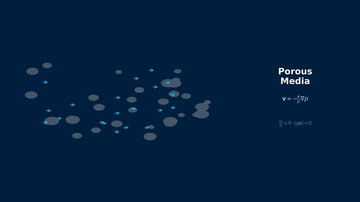
Theory: velocity proportional to pressure gradient
Overview
After an oil leak at a plant, I've been asked how many days it would take to reach a well 100 m away via groundwater. Where do I start?
Start with Darcy's law. When water seeps slowly through sand or soil, velocity is proportional to the hydraulic gradient (how steeply the water table slopes), with the proportionality set by the soil's hydraulic conductivity. Two cautions: Darcy velocity is an apparent value averaged over the whole cross-section, and the actual speed through the pores is that divided by porosity; and hydraulic conductivity varies by orders of magnitude between soils.
Darcy's law
$K$ is permeability (m², a property of the medium alone), $\mu$ viscosity, $k_h$ the hydraulic conductivity for water (m/s) and $i$ the hydraulic gradient. Hydrogeology tends to use hydraulic conductivity; petroleum and engineering use permeability, which is independent of the fluid and so convenient for comparing water and oil.
Estimating permeability (Kozeny–Carman)
$d$ is particle diameter and $\varepsilon$ porosity. The formula assumes a bed of uniform spheres; permeability scales with the square of particle size and depends strongly on porosity. Real soils with fines are usually less permeable than this predicts.
Pore velocity and validity
$v$ is the actual speed through the pores. When the particle Reynolds number $Re_d$ exceeds roughly 1–10, inertial drag adds and Darcy's law no longer holds.
The engineer who designed a fountain water supply
Darcy was a 19th-century French engineer who built a water supply bringing spring water to his home town of Dijon, with fountains throughout the city. In 1856 an appendix to his report described experiments passing water through vertical sand-filled pipes, showing that flow was proportional to head difference and inversely proportional to sand thickness. That was the birth of Darcy's law, and his name survives in the unit “darcy” (about 10⁻¹² m²). An appendix to a municipal water-works report became a basic law shared by groundwater hydrology, petroleum and chemical engineering.
Worked examples
Example 1: soil type and hydraulic conductivity
From Kozeny–Carman with porosity 0.35 and water at 20 °C:
| Material | Grain size | Permeability | Hydraulic conductivity |
|---|---|---|---|
| Fine sand | 0.2 mm | 2.3×10⁻¹¹ m² | 2.2×10⁻⁴ m/s (19 m/day) |
| Coarse sand | 1 mm | 5.6×10⁻¹⁰ m² | 5.5×10⁻³ m/s (477 m/day) |
| Gravel | 5 mm | 1.4×10⁻⁸ m² | 0.14 m/s |
Example 2: days to travel 100 m
| Material | Gradient | Darcy velocity | Pore velocity | Days for 100 m | Re_d |
|---|---|---|---|---|---|
| Fine sand | 0.01 | 2.2×10⁻⁶ m/s | 6.3×10⁻⁶ m/s | 183 days | 0.0004 |
| Coarse sand | 0.01 | 5.5×10⁻⁵ m/s | 1.6×10⁻⁴ m/s | 7.3 days | 0.06 |
| Gravel | 0.01 | 1.4×10⁻³ m/s | 3.9×10⁻³ m/s | 0.29 days | 6.9 |
| Gravel | 1.0 | 0.14 m/s | 0.39 m/s | — | 689 |
At the same gradient, half a year through fine sand but under half a day through gravel.
A 25-fold grain size gives 625 times the permeability. Also, pore velocity is about three times the Darcy velocity (1/0.35), so computing arrival time from Darcy velocity overestimates it threefold — always use pore velocity for contaminant arrival. And gravel under a steep gradient reaches a Reynolds number of 689, breaking Darcy's assumptions; use the Forchheimer equation there.
Example 3: effect of porosity error
For coarse sand (1 mm) relative to porosity 0.35, permeability is 0.54 times at 0.30 and 1.75 times at 0.40. A porosity difference of 0.05 changes permeability nearly twofold, so treat formula estimates as order-of-magnitude and use permeability test values for design. A coarse-sand filter 0.5 m² in area and 1 m deep under 1 m of head passes about 166 L/min.
How to approach the analysis
Cautions for CFD and groundwater models
- Porous-zone setup: many CFD codes specify porous media as a resistance coefficient (inverse permeability). Check units and whether superficial velocity is used.
- Layering: soil layers differ by orders of magnitude; a single average misses preferential paths through permeable layers.
- Anisotropy: horizontal and vertical conductivity often differ tenfold or more.
- Check validity: compute particle Reynolds numbers from the results and look for regions above 1–10.
“The well drew down less than expected”
A dewatering plan pumps from surrounding wells to keep groundwater out of an excavation, yet the water table falls less than expected — and the culprit turns out to be a thin gravel layer missed in the site investigation. Even a few tens of centimetres of gravel, with conductivity hundreds of times that of sand, can dominate the ground's overall transmissivity. The Darcy calculation is simple; the distribution of input conductivity decides almost everything. Read borehole logs carefully and include thin layers in the model.
Common mistakes
Mistakes and fixes
| Mistake | Effect | Fix |
|---|---|---|
| Arrival time from Darcy velocity | About 3× too slow | Use pore velocity (divide by porosity) |
| Confusing permeability and conductivity | Values off by about 10⁷ | Check units (m² vs m/s) |
| Using formula permeability for design | Errors of 2× or more | Confirm by permeability test |
| Omitting thin gravel layers | Preferential paths missed | Reflect borehole logs |
| Darcy's law at high velocity | Pressure drop underestimated | Check Re_d, use Forchheimer |
I'd like to compute permeability and velocity myself.
Try the permeability and Darcy's law tool for permeability and Darcy's law, and compare with pipe friction in the Darcy vs Fanning friction factor. Wall effects are covered in the Brinkman equation, and applications in packed beds and groundwater flow.
Related Topics
Experience the theory firsthand with the interactive simulator for this field
All Simulators