Forced Convection over a Flat Plate
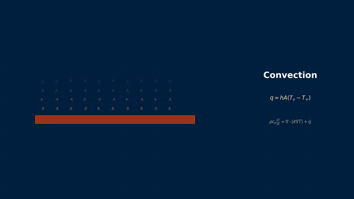
The Physics of Forced Convection over a Flat Plate
The Boundary Layer Is the Whole Story
When a uniform stream \( U_\infty \) flows along a flat plate, a velocity boundary layer develops near the wall in which the velocity climbs from zero to \( U_\infty \), together with a thermal boundary layer in which the temperature moves from the wall value \( T_w \) to the free-stream value \( T_\infty \). Essentially all of the resistance to heat transfer sits inside these thin layers, and the ratio of their thicknesses is set by the Prandtl number \( Pr = \nu/\alpha \) (air, \( Pr \approx 0.7 \): the two layers are of comparable thickness; oil, \( Pr \gg 1 \): the thermal layer is thinner; liquid metals, \( Pr \ll 1 \): the thermal layer is thicker). The flat plate is the reference problem of convective heat transfer — one of the few configurations where CFD, experiment, and correlation can all be laid side by side — which is why it also serves as a V&V validation benchmark.
Laminar Regime — the Blasius Solution and Local Nusselt Number
Below a critical value of the Reynolds number \( Re_x = U_\infty x / \nu \) built on the distance \( x \) from the leading edge (a working figure for a flat plate is \( Re_{x,c} \approx 5\times10^5 \), though free-stream turbulence shifts it substantially) the boundary layer is laminar, and the similarity (Blasius) solution yields the local Nusselt number for an isothermal wall with \( Pr \gtrsim 0.6 \).
$$ Nu_x = 0.332\, Re_x^{1/2} Pr^{1/3}, \qquad \overline{Nu}_L = 0.664\, Re_L^{1/2} Pr^{1/3} $$
The average is exactly twice the local value at \( x = L \) — the heat transfer coefficient peaks at the leading edge, where the boundary layer is thinnest, and decays downstream as \( x^{-1/2} \). For a uniform-heat-flux wall the coefficient 0.332 is replaced by 0.453. That the coefficient depends on the wall condition (isothermal versus uniform flux) is the first assumption to pin down whenever you compare CFD against a correlation.
Turbulent Regime and the Mixed Average
After transition the turbulent boundary layer transfers heat far more effectively. The representative local expression, and the mixed average that integrates across both the laminar and turbulent stretches, take the following form (assuming \( Re_{x,c} = 5\times10^5 \) and \( 0.6 < Pr < 60 \)).
$$ Nu_x = 0.0296\, Re_x^{4/5} Pr^{1/3}, \qquad \overline{Nu}_L = (0.037\, Re_L^{4/5} - 871)\, Pr^{1/3} $$
By convention every property is evaluated at the film temperature \( T_f = (T_w + T_\infty)/2 \). Even under ideal conditions these correlations carry roughly ±10–20% scatter, so treat them not as truth but as an experimentally grounded reference band.
Hand Calculation and CFD Practice
A Worked Hand Calculation — Air over a 0.5 m Plate
I follow the formulas, but I have no feel for what h actually comes out to with real numbers.
Push one case through by hand and it stays with you for life. Take air at an assumed film temperature of 50 °C (\( \nu \approx 1.8\times10^{-5} \) m²/s, \( k \approx 0.028 \) W/m·K, \( Pr = 0.70 \)), \( U_\infty = 10 \) m/s, and a plate length \( L = 0.5 \) m. First \( Re_L = 10 \times 0.5 / 1.8\times10^{-5} \approx 2.8\times10^5 \) — below the critical value, so the whole plate is laminar. The average Nusselt number is \( \overline{Nu}_L = 0.664 \times \sqrt{2.8\times10^5} \times 0.70^{1/3} \approx 0.664 \times 529 \times 0.888 \approx 312 \), giving an average heat transfer coefficient \( \bar{h} = \overline{Nu}_L\, k / L \approx 312 \times 0.028 / 0.5 \approx 17 \) W/m²K. For forced convection in air, h lands in the tens of W/m²K — once you carry that yardstick, a CFD run reporting h = 500 sets off the alarm the moment you see it.
Mesh and Wall Treatment in CFD
- Low-Re (wall-integrated) — first cell at \( y^+ \le 1 \), with 15–25 layers inside the boundary layer. The baseline setup for accurate heat transfer
- Wall-function — first cell placed at \( 30 \lesssim y^+ \lesssim 300 \). Coarser, but suited to large models. The intermediate band \( y^+ \approx 5\sim30 \) is the worst place to be: neither assumption holds and heat transfer goes badly off
- Inlet condition — free-stream turbulence intensity moves the transition location strongly. To compare against a correlation, either keep the intensity low (<1%) so a laminar stretch exists, or use a transition model (γ-Reθ and the like)
- Resolving the leading edge — refine in the streamwise direction as well near the leading edge, where the boundary layer is thinnest. Numerical smearing there propagates into the plate-average h
Using the Plate as a Validation Benchmark
The flat plate is the highest-value sanity test there is for a CFD setup. Overlay the local \( Nu_x \) distribution on the correlation and check three things: (1) is the \( x^{-1/2} \) slope reproduced in the laminar stretch, (2) does the transition location match expectation, (3) is the turbulent level within roughly ±10%. Carrying a setup that fails here — mesh, wall treatment, turbulence model — forward to a real geometry means that when the real geometry disagrees with measurement, you can no longer isolate the cause.
Guidance for Practical Work
Three Ways to Use the Correlations
- Sizing estimates — first-cut dissipation area and cooling airflow. Get the order of magnitude of the answer before touching CFD
- Cross-checking CFD — compare the average h from the analysis against the correlation; a factor of two or more apart means the setup is suspect
- Supplying boundary conditions — feed h to a conduction analysis or a 1-D thermal network as the heat transfer coefficient on faces you are not resolving in detail
Know Why Hardware Departs from the Correlation
| Factor | Effect | What to do |
|---|---|---|
| High free-stream turbulence (a few % on real machines) | Transition moves upstream and average h rises | Re-evaluate the mixed-average expression with a lower critical Re, or take the conservative fully turbulent form |
| An unheated starting length | The thermal layer develops late, raising h | Use the form with the unheated-starting-length correction |
| Surface roughness | Raises h in the turbulent stretch (smooth-wall expressions are the lower bound) | Move to a friction-coefficient-based rough-wall correlation |
| Finite width and edge effects | Three-dimensional flow makes h vary locally | Check with CFD when the width-to-length ratio is small |
| Temperature at which properties are evaluated | A large temperature difference turns property error into direct error | Evaluate strictly at the film temperature; add property-correction factors if needed |
Hardware Is Neither Isothermal nor Uniform-Flux
A real dissipating surface lies somewhere between the isothermal wall (the 0.332 family) and the uniform-heat-flux wall (the 0.453 family). The two differ by about 36% — meaning the idealisation of the wall condition alone carries a spread of that order. When accuracy matters, the right move is to go on to a conjugate heat transfer analysis coupled to conduction in the solid, keeping the correlation as a sanity check on the coupled result.
Handling in the Tools
Key Settings by CFD Tool
| Tool | Key points |
|---|---|
| Ansys Fluent | Enhanced Wall Treatment (y+-adaptive wall handling). Transition SST (γ-Reθ) for transition. Extract local Nu from the wall heat flux report |
| OpenFOAM | Wall functions via the nutkWallFunction family plus alphatWallFunction. For low-Re, mesh to y+<1 and drop the wall functions. Post-process with the wallHeatFlux utility |
| STAR-CCM+ | All y+ wall treatment. Transition model (Gamma ReTheta) built in. Extract the local h distribution with derived parts |
| COMSOL | Conjugate heat transfer interface for a single fluid-solid analysis. The laminar regime can be solved directly |
| 1-D / thermal network tools | Flat-plate correlations are built in with h computed automatically. Check the embedded assumptions (Re, Pr, wall condition) for the range of validity before relying on them |
Align the Definition of h Before Comparing Tools
The heat transfer coefficient is defined by \( h = q_w / (T_{ref} - T_w) \), but the choice of reference temperature \( T_{ref} \) — free-stream, adiabatic wall, or inlet temperature — can differ between a tool and a correlation. In high-speed flow where viscous heating matters, or in models mixing internal and external flow, that definitional gap manufactures apparent discrepancies of tens of percent. The safe way to compare across tools and against correlations is to work with the wall heat flux \( q_w \) itself, which carries no such definitional dependence.
Research Frontiers
Sharper Transition Prediction
Laminar-to-turbulent transition is the largest source of uncertainty in flat-plate heat transfer, and work continues on refining γ-Reθ-type models that judge transition from local variables alone, and on extending them to the sensitive environments (turbulence intensity, pressure gradient, roughness) that drive it. LES and DNS databases of the transition mechanisms — bypass transition, Tollmien-Schlichting waves — are now mature enough to serve as the calibration basis for RANS transition models. In practice the picture has not changed: error in the predicted transition location is the dominant contributor to error in the average h, so on any job where transition is in play, building a sensitivity study of the transition location into the standard workflow is the sound choice.
Extension to Non-Ideal Conditions
Data continue to accumulate, and correlations to be extended, for conditions closer to real hardware — highly turbulent free streams, rough surfaces, pulsating flow, combinations with impinging jets. Analytical and numerical solutions to conjugate Blasius-type problems, which build in the conjugate effect from the start (conduction within the plate sets the wall temperature distribution, which in turn feeds back into the boundary layer), are also being developed, so the escape from the isothermal-or-uniform-flux dichotomy is advancing on the theoretical side too.
Data-Driven Correlation Building
A growing body of work constructs heat transfer correlations from experimental and CFD data using symbolic regression or neural networks. These can potentially cover a wider range than the classical forms, but the risk of extrapolation and the need to guarantee physical consistency (dimensional consistency, limiting behaviour) remain open problems. The pragmatic middle ground — keep the dimensionless-group framework and let the data optimise only the coefficients and exponents — is the most promising landing point for practical use.
Troubleshooting
Symptoms, Causes, and Fixes
| Symptom | Likely cause | Fix |
|---|---|---|
| CFD Nu runs tens of percent above the laminar correlation | Unintended transition (turbulence intensity too high); unsuitable y+ | Lower the inlet turbulence intensity or use a transition model. Check the y+ distribution |
| CFD Nu falls well below the correlation | Under-resolved boundary layer (layer count, leading edge); wall function used outside its valid range | Redesign the boundary layer mesh. Switch to a low-Re treatment |
| Disagreement with experiment while CFD matches the correlation | Turbulence intensity, roughness, or edge effects on the experimental side | Re-check the dimensionless groups of the test conditions. Assess whether the gap sits within the uncertainty band |
| h differs by 20–30% between tools | Different definitions of the reference temperature | Compare on heat flux. Confirm the definitions in the documentation |
| Local Nu blows up near the leading edge | Discretisation of the leading-edge singularity (boundary layer thickness → 0) | Exclude values near the leading edge from evaluation (theory also gives Nu_x → ∞ there) |
| Hand calculation is off by an order of magnitude | Properties evaluated at the wrong temperature; wrong characteristic length (x versus L) | Re-evaluate properties at the film temperature. Check that local and average expressions have not been mixed up |
When in Doubt, Suspect Transition First
When CFD, the correlation, and the experiment all give different numbers, where should I start?
For a flat plate the prime suspect is the transition location. h differs by a factor of several between laminar and turbulent, so if the three sources do not agree on where transition happens, of course the numbers disagree. Diagnose it from the distribution: in CFD look at the streamwise \( x \) distribution of wall heat flux, in the experiment at the wall temperature distribution, and locate the position where h jumps — that is transition. Line up the transition location across all three, compare again, and the residual usually settles into the ±10–20% band of normal uncertainty. Before comparing values, compare the shape of the distribution — that is the iron rule of validating convective heat transfer.
Related: the Sieder-Tate correlation for internal flow, iterative coupling for conjugate heat transfer, how to read analysis results correctly.
Feel the theory hands-on with the interactive simulators in this field
Simulator LibraryRelated Fields
detail
error