Data Assimilation Methods
Data Assimilation Methods: Theoretical Foundations
Overview
Professor, I've heard of "Data Assimilation" in weather forecasting, but is it also used in CAE?
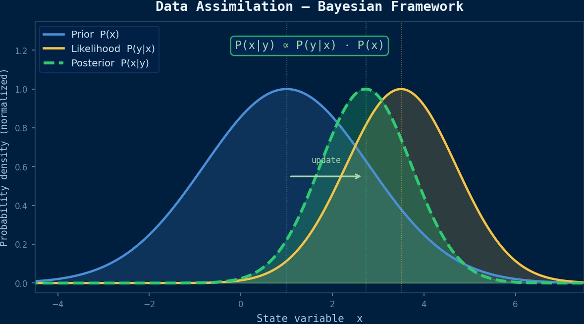
Exactly right. Data assimilation is a technique that statistically and optimally fuses simulation predictions with observational data to improve the accuracy of state estimation. In weather forecasting, atmospheric models and observation point data are fused to improve forecast accuracy. Similarly, in CAE, sensor data and FEM simulations can be combined to estimate the current state of a structure in real-time.
Isn't using just sensors enough?
Sensors only provide information from the locations where they are placed. Even if you attach 10 strain gauges to a bridge, you won't get information for tens of thousands of nodes. Using data assimilation, you can spatially interpolate and extrapolate limited sensor information using a simulation model to estimate the state of the entire structure.
Governing Equations
How is it formulated mathematically?
Let's explain it within the framework of the Kalman filter. The predicted value (from simulation) of the state vector $\mathbf{x}$ and the observed value are fused to obtain the analysis value (optimal estimate).
Here, $\mathbf{x}^f$ is the forecast value, $\mathbf{y}^o$ is the observed value, and $\mathbf{H}$ is the transformation operator from state space to observation space. The Kalman gain $\mathbf{K}$ determines the weighting between prediction and observation.
What are $\mathbf{P}^f$ and $\mathbf{R}$?
$\mathbf{P}^f$ is the forecast error covariance matrix (uncertainty of the simulation), and $\mathbf{R}$ is the observation error covariance matrix (uncertainty of the sensor). If the simulation is reliable, the Kalman gain becomes small, weakening the observation correction. Conversely, if sensor accuracy is high, more weight is placed on the observation side. This automatic weight adjustment is the essence of data assimilation.
Classification of Main Methods
Are there methods other than the Kalman filter?
Broadly speaking, there are two schools of thought.
- Sequential Methods: Ensemble Kalman Filter (EnKF). Represents forecast uncertainty using ensemble members in a Monte Carlo manner. Can handle nonlinear problems, but sampling error becomes an issue if the ensemble size is small.
- Variational Methods: 3D-Var/4D-Var. Minimizes the cost function $J(\mathbf{x}) = (\mathbf{x}-\mathbf{x}^f)^T\mathbf{B}^{-1}(\mathbf{x}-\mathbf{x}^f) + (\mathbf{y}^o-\mathbf{H}\mathbf{x})^T\mathbf{R}^{-1}(\mathbf{y}^o-\mathbf{H}\mathbf{x})$. 4D-Var also considers the time dimension.
Which one is used in CAE?
EnKF is more common in structural health monitoring. The FEM solver is run $N$ times (for the ensemble size) to estimate the forecast spread, which is then corrected with actual measurements. If the FEM is computationally expensive, techniques like combining it with reduced-order models (ROM) are necessary to reduce computational cost.
Kalman Filter—50 Years from Weather Prediction to Structural Analysis
At the theoretical heart of data assimilation is the Kalman filter (proposed in 1960). Originally developed for trajectory estimation in the Apollo program, this algorithm is now essential for numerical weather prediction. Japan's Meteorological Agency also utilizes it in its unique system combined with 4D-Var for typhoon track forecasting. Research applying this to CAE structural analysis surged in the 2010s. For example, an MIT research group published a method that sequentially assimilates full-field displacement data from a DIC camera attached to a material test specimen during an experiment using an ensemble Kalman filter, "identifying while measuring" parameters like Young's modulus and yield stress. The loop where "analysis complements experiment, and experiment corrects analysis" is the essence of data assimilation.
Computational Methods for Data Assimilation Methods
EnKF Implementation Steps
When implementing EnKF, what specific steps are taken?
Let's explain using structural analysis data assimilation as an example.
1. Initial Ensemble Generation: Create $N$ FEM models with uncertainties given to material parameters or load conditions ($N$ = 50~200 is a guideline).
2. Forecast Step: Execute FEM analysis for each ensemble member to obtain the state vector (displacement, stress, etc.).
3. Application of Observation Operator: Calculate "what would be seen if there were sensors" from each member's state.
4. Update Step: Calculate the Kalman gain and correct the entire ensemble using the difference from the actual observations.
5. Calculation of Statistics: The mean of the corrected ensemble becomes the optimal estimate, and its variance becomes the estimation uncertainty.
You run FEM 50 or even 200 times? Isn't the computational cost extremely high?
That's precisely why reducing computational cost is a major theme. There are three countermeasures.
- ROM Reduction: Use POD (Proper Orthogonal Decomposition) to reduce the FEM model to a lower dimension, speeding up the $N$ calculations.
- Localization: Limit the spatial influence range of the Kalman gain to cut unnecessary long-distance correlations.
- Inflation: Inflate the covariance to prevent the ensemble spread from becoming too small.
Variational Method Implementation
How is the variational method implemented?
4D-Var requires the adjoint equation of the FEM solver. The gradient of the cost function is efficiently calculated using the adjoint method, and optimization is performed using quasi-Newton methods (like L-BFGS). Implementing an adjoint solver is challenging, but it's a worthwhile investment as it can also be used for sensitivity analysis and inverse problems. However, many commercial FEM solvers don't have adjoint capabilities, so linking with automatic differentiation (AD) tools is a practical approach.
CAE Integration Pipeline
How do you integrate it into an existing CAE workflow?
Integration on Python is common. Control the FEM solver batch execution script, EnKF filtering logic, and sensor data acquisition/preprocessing with Python. Open-source data assimilation libraries like filterPy and DANEXT can serve as references.
| Component | Role | Tool Examples |
|---|---|---|
| FEM Solver | Forecast Calculation | CalculiX, Code_Aster, Abaqus |
| DA Framework | Filtering | filterPy, DAPPER, OpenDA |
| ROM Generation | Computational Cost Reduction | pyMOR, RBniCS |
| Visualization | Result Verification | ParaView, matplotlib |
Can it also do real-time processing?
With ROM reduction, filtering within a few seconds is possible. However, prior verification of whether the ROM's accuracy is sufficient compared to the full model is essential.
Ensemble Kalman Filter (EnKF)—Handling Uncertainty with Monte Carlo
The Extended Kalman Filter (EKF) assumes linear approximation, so it lacks accuracy for strongly nonlinear CAE problems. This is where the Ensemble Kalman Filter (EnKF) comes in. It generates tens to hundreds of "ensemble members" (sample states) from the initial state probability distribution, and each member is time-evolved through physical simulation while being sequentially corrected by observational data. A key point in implementation is choosing the ensemble size: if the size is too small, "sampling error" becomes large; if too large, computational cost explodes. In practical fluid analysis examples, the number of degrees of freedom × ensemble size often exceeds memory limits, and localization techniques to limit spatial correlation ranges are standard countermeasures.
Data Assimilation Methods in Practice
Application Procedure to Practical Work
Please tell me the steps for actually using data assimilation in a project.
First, select the target. Data assimilation is effective for cases where "you have a simulation model, but there are parameter uncertainties, and you want to correct them with limited sensor data."
1. FEM Model Construction: First, build an FEM model as usual and perform V&V under known load conditions.
2. Uncertainty Identification: Quantify the tolerances of material constants, load variation ranges, and uncertainties in boundary conditions.
3. Sensor Planning: Optimize where and how many sensors to place. Maximizing the information matrix can be an indicator.
4. DA Method Selection and Implementation: Choose between EnKF or variational methods based on computational cost and accuracy requirements.
5. Twin Experiment: First, generate "pseudo-observations" from simulation data to verify DA performance.
6. Application with Real Data: If no issues arise in the twin experiment, switch to real sensor data.
What is a twin experiment?
It's a test to try out DA performance in a situation where the true state is known. Run FEM with a certain parameter set to get the "true solution," add noise to those results to create pseudo-observations. Then verify the validity of the method by how close the values estimated by DA get to the true solution. This is a step you should always take before moving to real data.
Best Practices
What are the keys to success?
- Make the ensemble size sufficiently larger than the effective degrees of freedom of the state variables. If below 50, localization is essential.
- Set the observation error covariance $\mathbf{R}$ from sensor calibration information. Setting it arbitrarily can significantly distort results.
- When there is model bias (systematic error),