Digital Twins and ML
Digital Twins and ML: Theoretical Foundations
Overview
I hear about digital twins a lot lately, can you explain their relationship with CAE?
A digital twin is a technology that builds a virtual copy of a real-world physical system as a simulation model and monitors/predicts its state in real-time through synchronization with sensor data. By combining CAE physics models with machine learning, it enables fast prediction and adaptive updates.
How is it different from a regular CAE simulation?
The decisive difference is that it is "alive." A regular CAE simulation is run once during the design phase and that's it, but a digital twin continuously ingests sensor data and updates itself throughout its operational life. This enables predictions that account for aging degradation, unexpected loads, and environmental changes.
Governing Equations
How is it expressed mathematically?
It is formulated as a state-space model. The system state $\mathbf{x}_k$ follows a time evolution equation, and the observation $\mathbf{y}_k$ is its partial measurement.
Here, $f$ is the physics model (FEM, etc.), $\mathbf{u}_k$ is the input (loads, etc.), $\mathbf{w}_k$ is the model error, $h$ is the observation operator, and $\mathbf{v}_k$ is the observation noise. ML is used either as a fast approximation of $f$ (surrogate model) or for learning the model error $\mathbf{w}_k$.
What are the benefits of incorporating ML?
Using FEM's $f$ directly would be too slow for real-time updates. Approximating $f$ with ML enables predictions on the order of seconds. Furthermore, it can learn degradation mechanisms and environmental dependencies from data that are difficult to fully capture with physics models.
Physics-Informed Approach
How do you combine physics models and ML?
There are three patterns.
1. Hybrid Type: Corrects the physics model output with ML. $\hat{y} = f_{\text{physics}}(x) + f_{\text{ML}}(x, \text{residual})$
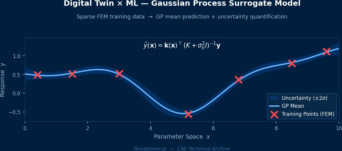
2. Surrogate Type: Replaces the entire physics model with ML. Fast but has challenges with extrapolation.
3. Physics-Constrained Embedded Type: Uses ML models with physical laws embedded in the loss function, like PINNs.
In practice, the hybrid type is the most reliable. It captures the global behavior with the physics model and corrects residuals with ML.
The Digital Twin Definition Debate—How "Alive" is the "Twin"?
Did you know the term "digital twin" actually has varying definitions depending on who you ask? The NASA-style definition is "a high-fidelity simulation that reflects the real-time state of the physical asset," but in manufacturing, the reality often stops at "a dashboard linking 3D CAD models with sensor data." To theoretically create a true digital twin, all four components—physics models, data assimilation, ML surrogates, and uncertainty quantification—must be in place. GE's gas turbine digital twin is among the most advanced, performing real-time assimilation of thousands of sensor signals per engine with over 300 FEM sub-models. However, it's said that maintenance costs alone reach hundreds of millions of yen annually, illustrating just how heavy a "true DT" can be.
Computational Methods for Digital Twins and ML
Implementation Architecture
How is a digital twin system configured?
Let's organize the main components.
| Layer | Component | Role |
|---|---|---|
| Data Acquisition Layer | IoT Sensors, SCADA | Real-time acquisition of temperature, strain, vibration, etc. |
| Communication Layer | MQTT, OPC-UA | Data transfer from sensors to cloud/edge |
| Model Layer | FEM + ROM + ML | Physics prediction and fast inference |
| Assimilation Layer | EnKF, Particle Filter | Model updating using sensor data |
| Visualization Layer | 3D Dashboard | State visualization and alerts |
How do you create a ROM?
POD (Proper Orthogonal Decomposition) is standard. Compute many full FEM solutions to form a snapshot matrix, then extract principal basis vectors via SVD. Even for a model with 1 million original degrees of freedom, 10-50 basis vectors often capture over 90% of the energy. This speeds up computation by tens of thousands of times.
ML Model Training and Updating
How do you create training data for the ML model?
A two-stage training process is common.
Offline Training: During the design phase, run many parametric FEM analyses to create a dataset of parameters and responses, and pre-train the ML model. Use Latin Hypercube Sampling (LHS) to efficiently cover the parameter space.
Online Training: After operation begins, update the model sequentially using actual sensor data. Use transfer learning or fine-tuning to adapt to small amounts of real data.
Is online training done in real-time?
Not necessarily real-time. In many cases, models are updated in batches daily or weekly. Real-time performance is needed for the data assimilation (state estimation) part, while model parameter updates themselves run on a slower cycle.
Edge Deployment Considerations
What if I want to run it on-site at the edge, not in the cloud?
Model lightweighting is key. Techniques include exporting to ONNX format and inferencing with ONNX Runtime, quantization (INT8) to reduce computation, and optimizing GPU inference with TensorRT. If the required computational load for inference is kept around 100 MFLOPS, millisecond-level response is possible even on edge devices like NVIDIA Jetson.
Surrogate Models Make Digital Twins "Fast"—FNO vs POD-ROM
What supports the real-time capability of digital twins are surrogate models (proxy models). Running full FEM at every step is computationally impossible, so lightweight approximation models are used for speedup. The classical method is POD-based ROM (Reduced Order Model), but it struggles with accuracy for strongly nonlinear problems. Gaining attention in the 2020s is the Fourier Neural Operator (FNO). The FNO from MIT×Caltech joint research is an architecture that learns "mappings from function to function," and there are cases where it achieved 1000x speed over conventional methods as a surrogate for the Navier-Stokes equations. A similar philosophy is adopted in Ansys SimAI, with demos showing CFD analyses that take hours being approximated in seconds.
Digital Twins and ML in Practice
Project Launch Steps
Where should I start a digital twin project?
Trying to go large-scale from the start leads to failure. A phased approach is the golden rule.
Phase 1: Proof of Concept (PoC) — Verify "whether predictions match actual measurements" using a single component, a few sensors, and a simple model. Duration: 3-6 months.
Phase 2: Pilot Operation — Accumulate data in the actual operational environment and gradually improve the model. Build the online learning mechanism. Duration: 6-12 months.
Phase 3: Full-Scale Deployment — Expand to multiple components and multi-physics support. Establish operation and maintenance systems.
Are there common patterns of failure in PoCs?
The most common is the "insufficient data" pattern. Sensor placement is inappropriate, sampling frequency is too low, or data quality is simply poor. It's crucial to plan the sensor strategy thoroughly before the PoC.
Best Practices
Please tell me the secrets to success.
- First, ensure the accuracy of the physics model. Even if you correct with ML, if the base physics model is sloppy, the whole thing falls apart.
- Perform regular sensor calibration. There's a risk of mistaking sensor drift for model degradation.
- Implement a mechanism to quantitatively monitor model prediction performance. Issue alerts if metrics like RMSE deteriorate.
- Strictly manage data versions. Traceability of data used for training, model versions, and inference results is necessary for audit compliance.
Application Examples
What are some concrete examples?
| Industry | Target | Effect |
|---|---|---|
| Aviation | Jet Engine Turbine Blades | Optimizes maintenance plans through remaining useful life prediction. |
| Wind Power | Wind Turbine Drive Train | Avoids unexpected shutdowns through failure precursor detection. |
| Bridges | Steel Bridge Fatigue Damage | Identifies damage locations by assimilating strain sensors and FEM. |
| Automotive | Battery Pack | Temperature distribution prediction and degradation monitoring. |
| Plant | Pressure Vessel | Online updating of creep life. |
Boeing 787 Digital Twin—Tracking the "Aging" of a Composite Airframe
Digital twins are being fully utilized in aircraft airframe maintenance management. The system Boeing deploys on the 787 links tens of thousands of channels of FDR (Flight Data Recorder) data recorded per flight with structural FEM simulations, tracking fatigue damage in composite outer panels based on each airframe's unique history. This enables a shift from the traditional "one-size-fits-all inspection schedule" to "individual schedules based on actual usage per airframe." The biggest implementation challenge was organizational: "Who updates the model?" The airframe design department, MRO (Maintenance, Repair, and Overhaul) department, and IT systems department operated in silos, making version management of simulators and maintaining consistency of data pipelines an organizational challenge beyond the technical aspects.