Aerodynamic Acoustic Analysis (FW-H Equation)
Aerodynamic Acoustic Analysis (FW-H Equation): Theoretical Foundations
Overview — What is the FW-H Equation?
Professor, what is the FW-H equation? I heard it's used to calculate noise from CFD results, but how does it work?
Good question. The FW-H equation is short for the "Ffowcs Williams-Hawkings equation," an acoustic analogy method published by John Ffowcs Williams and David Hawkings in 1969. Simply put, it's an extension of Lighthill's acoustic analogy to moving body surfaces.
I see... How is it used specifically? Doesn't CFD directly calculate all the sound?
That's the problem. Sound is a minute pressure fluctuation in the fluid, so trying to solve it directly with CFD all the way to far-field points leads to poor accuracy due to numerical dissipation and reflection effects. Moreover, the mesh would have to be extended to the observation points, causing computational costs to explode.
That's where FW-H comes in. CFD solves only the flow field near the object, and the far-field sound pressure is calculated post-processively using the FW-H integral equation. Thanks to this two-step approach, practical problems like aircraft jet noise, fan noise, and automobile side-mirror wind noise can be solved at realistic computational costs.
So it's used as a "post-processor" for CFD! That means the computational domain can be kept compact... But why can sound far away be determined by an integral?
Because the essence of sound is wave propagation. If the pressure and velocity fluctuations on the body surface (or a surrounding virtual surface) are known, the sound pressure at any far-field point can be calculated using the Green's function of the linear wave equation. This is precisely the principle of the FW-H integral.
Lighthill's Acoustic Analogy
Earlier you said it's "an extension of Lighthill's analogy." Could you first explain Lighthill's version?
Lighthill's acoustic analogy (1952) is the starting point of aeroacoustics. By transforming the Navier-Stokes equations, the following wave equation is derived:
Here, $\rho' = \rho - \rho_0$ is the density fluctuation, $c_0$ is the speed of sound in the uniform medium, and $T_{ij}$ is the Lighthill stress tensor, defined as:
What does $T_{ij}$ represent? Looking at the right-hand side, it includes momentum, pressure, viscous stress, and various other terms...
The key point is that the left-hand side has the form of the "wave equation in a stationary, uniform medium." The $T_{ij}$ on the right-hand side can be interpreted as an equivalent sound source. In other words, "all the actual turbulence is packed into the source term on the right, and the left side is treated as if it were sound propagation in a stationary fluid"—this is the essence of the analogy.
The dominant term in practice is $\rho u_i u_j$, which is the main cause of jet noise. It's also called the Reynolds stress tensor. At low Mach numbers, the other terms become small, so it can be approximated as $T_{ij} \approx \rho_0 u_i u_j$.
I see, so turbulence is reinterpreted as a "sound source," hence "analogy." But doesn't this lack the effect of the body surface?
Sharp observation. That's correct; Lighthill's original formulation targets turbulence in free space. To handle surface effects of rotating fan blades or flying aircraft, boundary conditions need to be incorporated into the integral. That is the FW-H equation.
FW-H Equation Formulation
Finally, the FW-H equation itself. What form does it take?
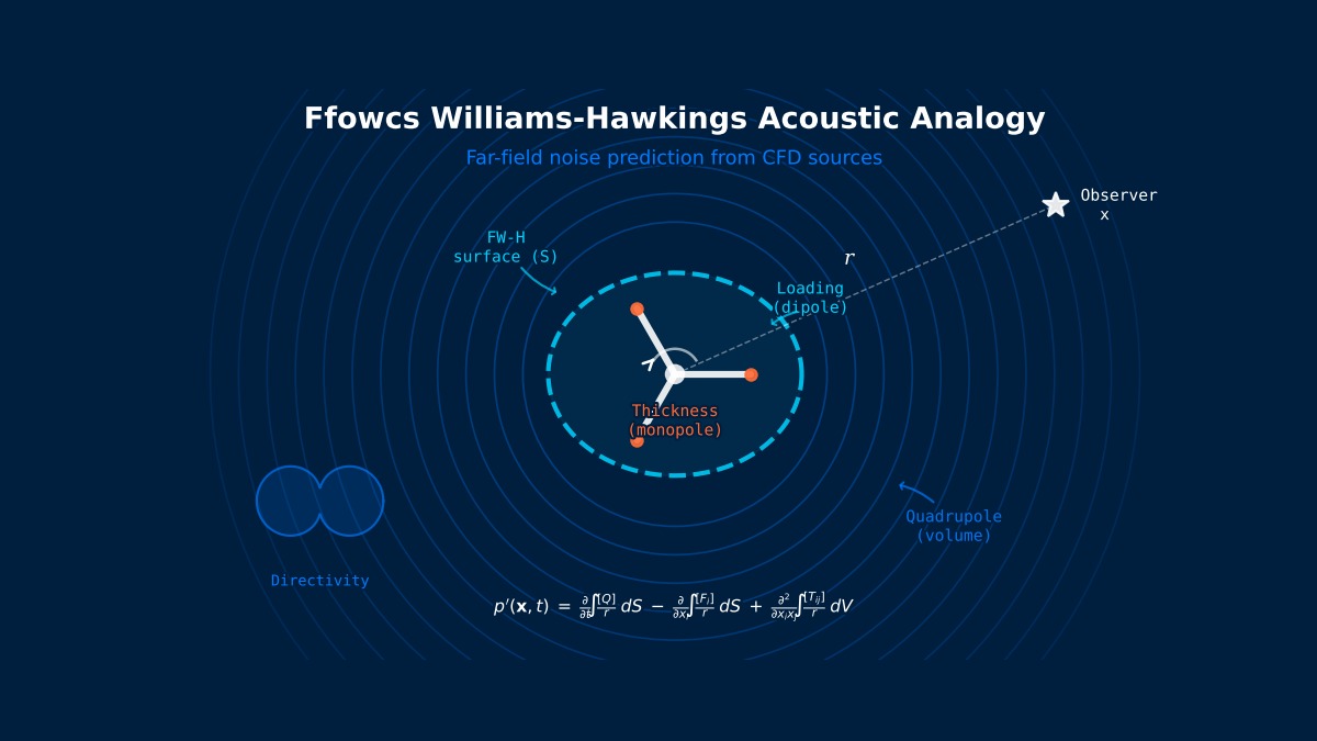
The FW-H equation extends Lighthill's equation to a moving body surface $f=0$ using generalized functions (Heaviside function, Dirac delta function). As a result, the far-field sound pressure fluctuation $p'(\mathbf{x},t)$ is expressed as the sum of three terms:
Here, $[\cdot]_{\mathrm{ret}}$ means evaluation at the retarded time, $r$ is the distance from the source point to the observation point, $M_r$ is the Mach number component of the source in the observation direction, $v_n$ is the surface normal velocity, and $\ell_i = (p\delta_{ij} - \tau_{ij})n_j + \rho u_i(u_n - v_n)$ is the load vector.
Physical Meaning of the Three Source Terms
Wow, there are three terms... What kind of sound does each represent specifically?
Alright, let me explain each one with examples.
1. Thickness Noise: When an object moves, air is pushed away in front and pulled in behind. This is the effect of the blade's "thickness" periodically pushing air when a helicopter blade rotates. It appears as discrete tones at integer multiples of the rotation frequency × number of blades (BPF: Blade Passing Frequency).
2. Loading Noise: The pressure acting on the object surface (fluctuations in lift and drag) becomes the sound source. When fan blades interact with the wake and lift fluctuates, this generates sound. For an automobile side mirror, pressure fluctuations on the mirror surface transmit into the cabin as a "whoosh" wind noise.
3. Quadrupole Noise: Sound emitted by the turbulence itself in the space outside the object. A typical example is the broadband "roar" from a jet engine exhaust plume. It requires a volume integral and is computationally expensive. However, at low Mach numbers (around $M < 0.3$), it is small compared to thickness and loading noise, so it is often omitted in practice.
I see! So for low-speed vehicles or fans, the two surface integral terms are mostly sufficient, and for high-Mach-number problems like jet engines, the quadrupole term also becomes significant.
Exactly. In fact, in implementations of FW-H in Ansys Fluent or STAR-CCM+, only the thickness and loading surface integrals are enabled by default, with the quadrupole term being optional.
Permeable Surface Formulation
I sometimes hear about "permeable surfaces." Do you use a virtual surface instead of the object surface?
This is a very important practical technique. The original FW-H equation takes the integration surface as the object surface (solid surface), but in the permeable surface formulation proposed by di Francescantonio (1997), a virtual closed surface (permeable surface) surrounding the object is used as the integration surface.
There are two benefits. First, it avoids the volume integral for the quadrupole. If the permeable surface is taken large enough to enclose the source region, the quadrupole contribution can also be captured with just a surface integral. Second, nonlinear flow effects (such as high-Mach-number flows including shock waves) can also be incorporated as surface data.
So using a permeable surface solves everything? Are there no drawbacks?
Unfortunately, vortices passing through the permeable surface can generate spurious noise. Especially when a jet flow crosses the downstream edge of the permeable surface, the sound calculated inside and outside the surface fails to cancel properly, resulting in non-physical low-frequency noise. This is called the end-cap problem. Surface placement requires a craftsman's know-how.
The Two Geniuses Who Created the FW-H Equation
John Ffowcs Williams (born in Wales, Cambridge University professor) is called the "father of aeroacoustics" and became famous for his research on Concorde jet noise. His collaborator David Hawkings was a graduate student at the time; their 1969 paper published in Philosophical Transactions became the foundation for aeroacoustic analysis for over 50 years. Meanwhile, Sir James Lighthill, who laid the theoretical groundwork, is a giant in fluid dynamics in general; his 1952 paper on acoustic analogy has been cited over 10,000 times. Interestingly, the theory Lighthill proposed in 1952 was a revolutionary idea at a time when noise testing for a single jet engine cost hundreds of millions of yen: "predicting noise through calculation."
Computational Methods for Aerodynamic Acoustic Analysis (FW-H Equation)
Time-Domain Integration Method (Farassat 1A)
How do you actually solve the FW-H equation on a computer? Do you numerically integrate that integral directly...?
The most widely used method in practice is the Farassat 1A formulation. It's a closed-form expression for the solution of the FW-H equation in the time domain, derived by NASA's Farassat in the 1980s.
The contribution of the thickness source is:
The contribution of the loading source is:
Calculating the retarded time seems tough. You have to compute the sound travel time from each surface element to the observer...
That's the crucial part of implementing an FW-H code. For each surface element, the retarded time $\tau$ is found from the following equation:
This implicit equation is solved iteratively using Newton's method. It can be solved analytically in a uniform flow, but modifications are needed when mean flow effects are present. Many commercial software packages adopt fast algorithms assuming uniform flow.
Frequency-Domain Method
Are there approaches other than the time domain?
There is also a method to solve the FW-H equation in the frequency domain. The pressure/velocity data on the surface is decomposed into frequency components via FFT, and integration is performed for each frequency using the Green's function of the Helmholtz equation.
The advantage is efficiency when only specific frequency bands need to be calculated. The disadvantage is the need to store a large amount of unsteady data in the time direction. In practice, it is well-suited for analyzing tone noise from rotating machinery (BPF components).
CFD Coupling Flow
Regarding the coupling between CFD and FW-H, what kind of data exchange happens specifically?
A typical flow is as follows:
- Run a CFD unsteady calculation and record pressure $p$, density $\rho$, and velocity $\mathbf{u}$ on the FW-H surface at each time step.
- Once sufficient statistics are obtained (typically tens to hundreds of flow-through times), pass the recorded data to the FW-H solver.
- The FW-H solver calculates the sound pressure time history $p'(t)$ at each observer point.
- Perform FFT on the sound pressure time history to compute the spectrum (SPL vs. frequency) and OASPL (Overall SPL).
In Ansys Fluent or STAR-CCM+, an "on-the-fly" mode that executes the FW-H integral simultaneously with the CFD calculation is also available. It saves memory, but the drawback is that observer positions cannot be changed afterward.
Turbulence Model Selection
What turbulence model should be used on the CFD side? Is something like the k-ε model okay?
RANS (k-ε, k-ω SST, etc.) cannot be used for aeroacoustic analysis. This is a very important point. RANS solves the time-averaged flow field, so it cannot resolve the instantaneous pressure fluctuations that become sound sources.
What is needed for aeroacoustics is:
- LES (Large Eddy Simulation): Directly resolves large-scale eddies and approximates small scales with an SGS model. Most reliable but computationally expensive.
- DES/DDES (Detached Eddy Simulation): A hybrid method that uses RANS near walls and LES in separated regions. Offers a good practical balance.
- SAS (Scale-Adaptive Simulation): Menter-Egorov model. URANS-based but capable of LES-like resolution.
For example, for automobile side-mirror wind noise, DDES + FW-H has become the practical standard. For fan noise, LES is preferred; for jet plume noise, LES is desirable but DDES is also used due to computational cost.
Mesh and Time Step Requirements
When calculating sound, are the mesh requirements stricter than for regular CFD?
Exactly. Guidelines for the resolution required for aeroacoustics:
Related Topics
Experience the theory with interactive simulators in this field
Standing Wave Simulator All SimulatorsRelated fields
| Parameter | Recommended Value | Remarks |
|---|---|---|