Thermal Shock Analysis — Crack Initiation Due to Rapid Temperature Changes and the Role of the Biot Number

Good question. The Biot number is the ratio of the internal conductive thermal resistance to the external convective thermal resistance at the surface. The formula is

That depends heavily on the material's brittleness. For example, in brittle materials like ceramics (Al₂O₃, k=30 W/(m·K)), conditions where Bi exceeds 1, such as a thin-walled component (Lc=0.01m) exposed to high-temperature gas (h=1000 W/(m²·K)), can enter the danger zone even at

The essential difference is the presence of the time derivative term. Since time variation is everything in thermal shock, the non-steady (transient) Fourier equation is used.

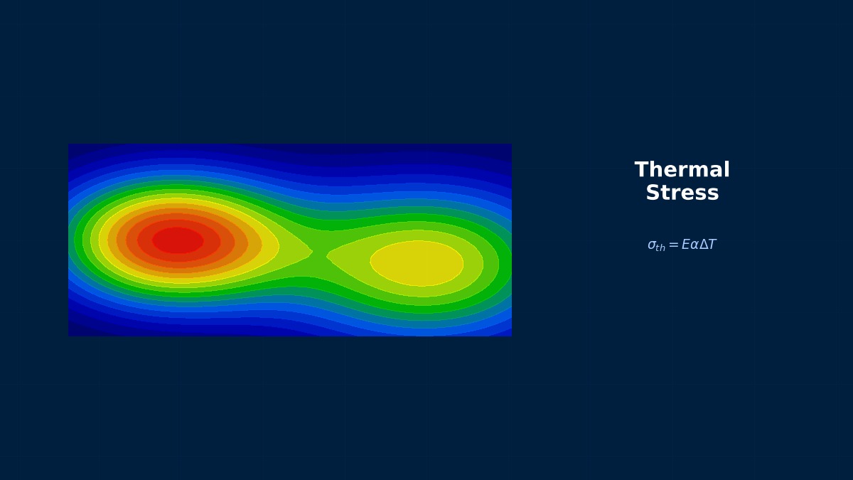
We use the constitutive law (Hooke's law) that considers thermal strain. For isotropic materials, the thermal stress σ_th is related as follows:

To capture rapid changes like thermal shock, unconditionally stable implicit methods (e.g., backward difference method) are essential. Explicit methods have strict stability conditions (CFL condition) on the time step Δt, making computational costs enormous for meshes with small elements. With implicit methods, a system of linear equations is solved at each time step:

For the initial phase of thermal shock (the moment of rapid temperature change), automatic time stepping should be used. For example, in Ansys, set the initial, minimum, and maximum steps with "DELTIM". As a guideline, set the minimum step to 1/10 or less of the time it takes for heat to propagate through the characteristic length Lc. With thermal diffusivity α=k/(ρc_p),

Matching meshes is ideal but not mandatory. Many solvers have functions to map (interpolate) results between different meshes. However, accuracy loss can indeed occur. Particularly in areas with steep temperature gradients caused by thermal shock, if the structural mesh is too coarse, thermal strain can be underestimated. The countermeasure is to sufficiently refine both meshes in areas with large temperature gradients (surface, crack tip) and increase the element order. In Abaqus, mapping can be controlled using "*TIE" or "*COUPLING". To evaluate mapping error, a verification analysis should be run comparing nodal temperatures from the thermal analysis mesh with those from the mapped structural mesh nodes.

The following 6 steps are practical.
1. **Define Prerequisites**: Determine the maximum temperature difference ΔT_max, heat transfer coefficient h, and exposure time t_exp from specifications or experiments. Calculate the Biot number to understand the problem's scale.
2. **Geometry & Mesh**: Especially refine the mesh for the surface layer where temperature gradients are large. Boundary layer meshing is effective. Have at least 5 elements in the thickness direction.
3. **Material Settings**: Input temperature dependencies (k, c_p, α, E, ν) as much as possible. If high-temperature material data is unavailable, refer to databases like JAHM (Japan High Temperature Materials Database).
4. **Boundary Conditions**: To reproduce thermal shock, apply surface heat transfer coefficient as a step or steep function. Consider combined convection and radiation.
5. **Analysis Execution**: Perform one-way coupled analysis in the order: transient heat conduction → static structural. Use automatic time stepping.
6. **Post-processing**: Extract the time and location of maximum thermal stress, temperature history, and time variation of thermal stress.

At a minimum, verify the following 4 points.
**1. Energy Balance**: Is the error in the heat energy balance output by the solver (input heat vs. internal energy increase + dissipated heat) within 1%? In Ansys, check with the "PRENERGY" command.
**2. Mesh Dependency**: Is the difference in maximum thermal stress between the finest mesh (baseline mesh) and the next coarser mesh within 5%? Especially verify by changing the surface mesh size.
**3. Time Step Dependency**: When the minimum time step is halved, do the peak temperature and stress values remain unchanged?
**4. Comparison with Simplified Theoretical Values**: For example, estimate the temperature difference ΔT_s-c between the surface and center of a plate using a simplified formula (constant heat flux approximation) like

Since cracks initiate due to tensile stress, the first principal stress (σ1) is most important. Evaluate in the following order.
1. **Location and Time of Maximum Tensile Stress**: In the transient analysis, does σ1 exceed the material's tensile strength (e.g., the four-point bending strength from JIS R 1606 for ceramics)? If it exceeds, the risk of crack initiation is high.
2. **Stress Gradient**: The distribution becomes tensile at the surface and compressive inside. The depth of this tensile stress region serves as an indicator for potential crack penetration depth.
3. **Thermal Stress Concentration Factor**: At geometric corners or hole edges, the theoretical thermal stress is multiplied by a shape factor (Kt). Calculate the effective Kt by dividing the maximum stress from FEM by the nominal thermal stress from plate theory.
4. **Fracture Mechanics Parameters**: If assuming an initial defect, evaluate the stress intensity factor KI at its location using methods like the J-integral, and compare it with the material's fracture toughness KIC (from standards like ASTM E399).

It depends on the purpose. **Ansys Mechanical** has a well-established workflow, especially the one-way coupling of "Steady-State Thermal" → "Transient Thermal" → "Static Structural" is straightforward. Advanced control is possible using APDL scripts. **Abaqus/Standard** excels at fully coupled two-way analysis (considering thermal-structural interaction) using the *COUPLED TEMPERATURE-DISPLACEMENT analysis step. Abaqus is advantageous for problems involving plastic heat generation or frictional heating. **COMSOL Multiphysics** has intuitive GUI settings for coupling and can solve heat conduction and solid mechanics simultaneously as a single "physics." It's fast for prototyping and parameter studies.

There's no major difference, but the data input formats vary.
- **Ansys**: Input in Engineering Data as a table with temperature as the independent variable. Define k, c_p, α, E, ν, etc., individually. In APDL, use the "MPTEMP" and "MPDATA" commands.
- **Abaqus**: Use "Depvar" in Material Properties or program with user subroutines like "USDFLD" or "UMAT". More suitable for complex dependencies (like annealing effects).
- **COMSOL**: Has a rich material library with temperature-dependent data for many materials pre-loaded. Setting custom functions (analytic, interpolation) via GUI is simple.
For all, a key tip for accuracy is to provide data points at least every 100°C, with 5 or more points. Be especially careful with ceramics, as their specific heat c_p has significant temperature dependence.

It's possible, but preprocessing and setup require more effort. **Code_Aster** (in the Salome-Meca environment) is very powerful and can execute coupled transient heat conduction (THER_NON_LINE) and thermal stress (MECA_STATIQUE) analysis. It can handle material temperature dependency and nonlinearities. The issue is that all settings must be written in a command file (.comm), resulting in a steep learning curve. **CalculiX** is similar. The user must consciously set the mesh quality checks and solver stabilization defaults that commercial software GUIs handle automatically. They are good for small-scale studies or educational purposes, but for obtaining reliable results quickly in practical design, commercial software's completeness and support are still advantageous.

Three main causes are possible.
1. **Steep Boundary Conditions**: Applying the heat transfer coefficient h as a step function makes the initial temperature change rate approach infinity, causing numerical instability. As a countermeasure, apply it as a linear or exponential function with a realistic rise time (e.g., 1 millisecond). In Ansys, use the "Function" tool.
2. **Discontinuous Material Properties**: In the temperature dependency data table, material values jump too much between adjacent temperature points (e.g., k=50 at 100°C, k=10 at 101°C). Smooth the data or input it at finer temperature intervals.
3. **Inappropriate Time Step**: Even with implicit methods, extremely large time steps can cause non-physical oscillations. Limit the "maximum step" in automatic step control to the order of the thermal time constant (Lc²/α).

It's highly likely you are mistaken about the **constraint conditions** or the **evaluation time**. First, check if deformation due to thermal expansion can occur freely. If the entire object is completely fixed, areas with temperature increase will be entirely compressed. In thermal shock, the cold interior acts as a "constraint," suppressing the expansion of the heated surface, which puts the surface in tension. To reproduce this mechanism, correctly apply boundary conditions like symmetry to the model, restraining only rigid body motion. Next, consider at which time step of the transient analysis you are looking at the stress. Immediately after thermal shock, the surface heats up and tries to expand, so it might temporarily become compressive. Later, as heat propagates inward, the balance changes. It is essential to check the stress time history with animation.

That is a typical symptom when a **geometric singularity** (sharp corner, crack tip) exists. In linear elastic analysis, as the tip's curvature radius approaches zero, the theoretical stress diverges to infinity. With FEM, refining the mesh brings the value closer to that infinity, so it doesn't converge. There are two countermeasures.
1. **Modify to Realistic Geometry**: Perfect sharp corners don't exist in design. Incorporate the manufacturing fillet radius (e.g., R0.1mm) into the model. This alone will make the stress concentration factor settle to a finite value.
2. **Adopt a Fracture Mechanics Approach**: If the existence of a crack is a premise,