Potential Flow Theory
Potential Flow Theory: Theoretical Foundations
What is Potential Flow?
Professor, what is potential flow? It's also called irrotational flow, right?
Potential flow is an inviscid, irrotational (zero vorticity) flow. If the vorticity is zero, the velocity field can be expressed as the gradient of a scalar potential $\phi$.
Substituting this into the incompressible continuity equation $\nabla \cdot \mathbf{u} = 0$ yields the Laplace equation.
The Laplace equation appears in many different fields, doesn't it?
Exactly. Many physical phenomena, such as electrostatic fields, steady-state heat conduction, and groundwater flow, reduce to the Laplace equation. The theory of potential flow is mathematically equivalent to these fields.
Basic Flow Elements
Since the Laplace equation is linear, its solutions can be superimposed, right?
Excellent point. That's the greatest strength of potential flow theory. Complex flows can be constructed by superimposing basic flow elements.
| Flow Element | Velocity Potential $\phi$ | Stream Function $\psi$ | Physical Meaning |
|---|---|---|---|
| Uniform Flow (x-direction) | $U_\infty x$ | $U_\infty y$ | Freestream flow far away |
| Source (strength $m$) | $\frac{m}{2\pi}\ln r$ | $\frac{m}{2\pi}\theta$ | Fluid emission from a point |
| Vortex (circulation $\Gamma$) | $\frac{\Gamma}{2\pi}\theta$ | $-\frac{\Gamma}{2\pi}\ln r$ | Rotation around a point |
| Doublet (strength $\mu$) | $-\frac{\mu \cos\theta}{2\pi r}$ | $-\frac{\mu \sin\theta}{2\pi r}$ | Limit of source + sink |
What happens if you combine a source and a uniform flow?
You get a Rankine half-body. Placing a source of strength $m$ in a uniform flow $U_\infty$ creates a stagnation point at $(x,y) = (-m/(2\pi U_\infty), 0)$, and the streamline passing through it forms the body surface.
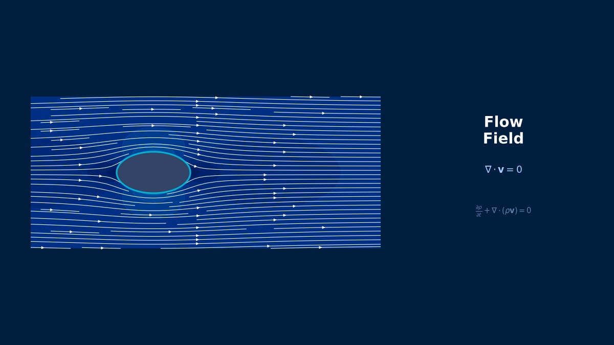
Flow Around a Cylinder
The most famous example is flow around a cylinder, right?
The potential flow around a cylinder of radius $a$ in a uniform flow $U_\infty$ is obtained by superimposing a doublet and a uniform flow.
The surface velocity (at $r=a$) is $u_\theta = -2U_\infty \sin\theta$, reaching a maximum value of $2U_\infty$ at $\theta = \pi/2$ (the top).
You can also get the pressure distribution using Bernoulli's theorem, right?
The pressure coefficient becomes $C_p = 1 - 4\sin^2\theta$. This leads to the famous d'Alembert's paradox. Since the pressure distribution is symmetric fore and aft, drag becomes zero in inviscid potential flow.
Kutta-Joukowski Theorem and Lift
Drag is zero, but can lift be generated?
Adding circulation $\Gamma$ around the cylinder generates lift. Adding a vortex to the velocity potential:
According to the Kutta-Joukowski theorem, the lift per unit span is
The magnitude of the circulation determines the lift. For airfoils, the Kutta condition (the condition that the flow leaves the trailing edge smoothly) uniquely determines the value of the circulation.
This theorem is the foundation of airfoil design, right?
Exactly. Using the Joukowski transformation, one can analytically find the flow around an airfoil from the cylinder solution. It's a theory that can be considered the starting point of aeronautical engineering.
Scope of Application and Limitations
In what cases is potential flow theory effective?
It provides a good approximation under the following conditions.
- High Reynolds Number: When viscous effects are confined to the boundary layer
- Regions Far from the Body: Vorticity is nearly zero outside the boundary layer
- Flows Without Separation: Such as airfoils at small angles of attack (before stall)
- Steady or Quasi-Steady: Conditions without vortex shedding
Conversely, it is not applicable to flows involving separation, low Reynolds numbers, or strongly unsteady vortex flows. In actual CFD, the Navier-Stokes equations are solved, but potential flow theory still plays an active role in rapid evaluation during the initial design stage and in validating the reasonableness of CFD results.
D'Alembert's Paradox—The Contradiction of "Zero Drag"
In the 18th century, Jean le Rond d'Alembert used potential flow theory to prove that "the drag on a body moving in an ideal fluid is zero." This is called "d'Alembert's paradox." In reality, it is obviously not zero—this contradiction remained unsolved for over 100 years, hindering the development of fluid mechanics. The solution was Prandtl's boundary layer theory (1904). The answer is that "even a tiny amount of viscosity changes the pressure distribution through a thin boundary layer, generating drag." The behavior at the limit (viscosity→0) is completely different from the solution for zero viscosity—this concept of "singular perturbation" remains an important theme in mathematics and physics today.
Computational Methods for Potential Flow Theory
Basics of Panel Method
How do you solve potential flow numerically?
The most widely used method is the Panel Method. The body surface is divided into panels (line segments or surface elements), and singularities (sources, doublets, vortices) are placed on each panel. It's a method that discretizes the boundary integral equation to find the strength of the singularities.
Here $G$ is the Green's function (in 2D, $G = -\frac{1}{2\pi}\ln|\mathbf{x}-\mathbf{x'}|$), $\sigma$ is the source strength, and $\mu$ is the doublet strength.
Compared to solving the N-S equations in 3D space, the computation is completed only on the surface, right?
That's the biggest advantage of the panel method. A 3D problem reduces to a 2D surface problem, drastically reducing computational cost. Mesh generation also only requires a surface mesh.
Hess-Smith Panel Method
Please teach me the most basic panel method algorithm.
The Hess-Smith Panel Method is used for flow around bodies without lift. The algorithm is as follows.
1. Divide the body surface into $N$ panels
2. Place a constant-strength source $\sigma_j$ on each panel
3. Impose the condition that the normal velocity = 0 at each panel's control point (midpoint)
4. Solve the $N \times N$ system of equations $[A]\{\sigma\} = \{b\}$
5. Calculate the tangential velocity on each panel and find the pressure using Bernoulli's equation
The influence coefficient matrix $A_{ij}$ is the normal velocity component induced at panel $i$'s control point by the source on panel $j$.
How do you calculate lift?
Add vortex panels to Hess-Smith. Add a vortex distribution $\gamma$ to each panel and add the Kutta condition (equal velocities on the upper and lower panels at the trailing edge) to the system of equations. This yields the circulation and lift.
Higher-Order Panel Methods
How can accuracy be improved?
The basic Hess-Smith assumes a constant (zeroth-order) singularity distribution on each panel, but there are the following improvements.
| Panel Method Type | Singularity Distribution | Accuracy | Computational Cost |
|---|---|---|---|
| Constant Panel (Hess-Smith) | Constant | 1st order | Low ($O(N^2)$) |
| Linear Panel | Linear distribution | 2nd order | Medium ($O(N^2)$) |
| Quadratic Panel | Quadratic distribution | 3rd order | High ($O(N^2)$) |
| High-Order Panel + FMM | Arbitrary | High order | $O(N \log N)$ or $O(N)$ |
So computational cost can be reduced with FMM.
Combining with FMM (Fast Multipole Method), which calculates the influence of distant panels collectively using multipole expansions, can reduce computational cost to $O(N)$. This is an essential technique for 3D full-aircraft analysis where the number of panels reaches tens to hundreds of thousands.
Representative Panel Method Codes
Related Topics
Experience the theory firsthand with the interactive simulator for this field
All Simulators