How does the finite volume method differ from the finite element method?

The finite volume method divides the domain into small control volumes and enforces the conservation law as a balance of fluxes through each control volume's faces. Because neighbouring cells share the same face flux, mass and momentum are conserved exactly at the discrete level, which is why most general-purpose CFD codes use it.

Why does central differencing oscillate?

When the cell Péclet number (the ratio of convection to diffusion) exceeds 2, some coefficients of the central scheme become negative and the solution develops unphysical wiggles. In the 1D example, a cell Péclet number of 5 pushed the value up to 2.46. Refine the mesh or use an upwind-type scheme.

Is first-order upwind safe?

It does not oscillate, but numerical diffusion smears gradients. In the 1D example, doubling the mesh reduced the error by only about 1.7×. Final results are normally computed with a second-order scheme, with first-order upwind reserved for start-up stabilisation.

Finite Volume Method Fundamentals

Category: Fluid Analysis (CFD) | Revised 2026-09-28

CAE visualization for fvm fundamentals theory - technical simulation diagram

Fundamentals of the Finite Volume Method

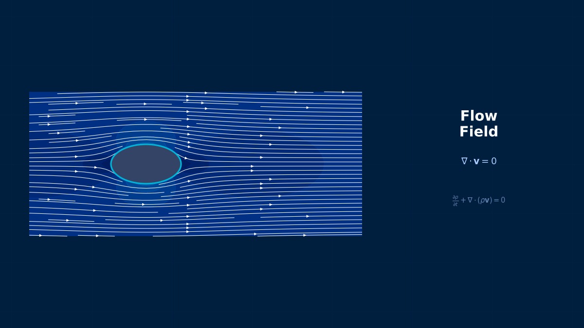
Theory: conservation as a balance over boxes

Overview

🙋

I hear almost every CFD code uses the finite volume method. What makes it so different from the finite element method we use for structures?

🎓

They start from different ideas. FEM multiplies the differential equation by weight functions and integrates over the whole domain (the weak form). FVM cuts space into small boxes — control volumes, or cells — and writes the balance directly: the rate of change inside a box equals what flows in through its faces minus what flows out, plus any source. Neighbouring boxes exchange exactly the same amount through their shared face, so mass cannot silently appear or vanish anywhere. That is the main reason it is preferred for fluid flow.

The integral transport equation

For a quantity $\phi$ (a velocity component, temperature, concentration, …) in a field with density $\rho$, velocity $\mathbf{u}$ and diffusivity $\Gamma$, conservation over a control volume $V$ with surface $S$ reads:

$$ \frac{\partial}{\partial t}\int_V \rho\phi\, dV + \oint_S \rho\phi\, \mathbf{u}\cdot d\mathbf{S} = \oint_S \Gamma \nabla\phi \cdot d\mathbf{S} + \int_V S_\phi\, dV $$

From left to right: unsteady, convection, diffusion and source terms. Replacing the surface integrals by sums over the faces $f$ of cell $P$ gives the discrete equation ($N$ is the neighbour across the face and $F_f$ the mass flux through it):

$$ \frac{(\rho\phi)_P^{n+1}-(\rho\phi)_P^{n}}{\Delta t} V_P + \sum_{f} F_f\, \phi_f = \sum_{f} \Gamma_f \frac{\phi_N-\phi_P}{|\mathbf{d}|}|\mathbf{S}_f| + S_\phi V_P, \qquad F_f = (\rho\, \mathbf{u}\cdot\mathbf{S})_f $$

🙋

The equation looks simple. Where is the hard part?

🎓

The unknowns live at cell centres, but the equation needs face values $\phi_f$ and face gradients. How you interpolate from centres to faces largely decides accuracy and stability, and that is what the next sections are about.

Cell-centred and vertex-centred layouts

Layout	Where unknowns live	Typical use
Cell-centred	Cell centres; each cell is a control volume	OpenFOAM, Ansys Fluent, Simcenter STAR-CCM+
Vertex-centred	Mesh vertices, with a dual cell built around each vertex	e.g. Ansys CFX

Coffee Break Trivia

The book that spread heat-and-flow computing

S. V. Patankar's textbook “Numerical Heat Transfer and Fluid Flow” (1980) is often credited with bringing the finite volume method into engineering practice. It showed, step by step, how to assemble discrete equations from control-volume balances, together with the SIMPLE algorithm for correcting pressure and velocity alternately (published by Patankar and Spalding in 1972). Much of what runs inside today's commercial codes is a continuation of that book.

Discretisation: choosing face values

Diffusion: central differencing and non-orthogonal correction

The face gradient in the diffusion term is basically $(\phi_N-\phi_P)/|\mathbf{d}|$, the difference between the two cell centres. That is exact only when the vector $\mathbf{d}$ joining the centres is normal to the face. On non-orthogonal meshes a correction built from cell-centre gradients is added, usually treated explicitly, so strongly non-orthogonal meshes tend to make the iterations unstable.

Convection: choosing a scheme

Scheme	Order	Behaviour
First-order upwind	1st	Always bounded and robust; strong numerical diffusion smears gradients
Central differencing	2nd	Oscillates when the cell Péclet number exceeds 2
Second-order (linear) upwind	2nd	Extrapolates with the upstream gradient; the practical default; can overshoot slightly
QUICK	3rd (uniform grid)	Accurate but not guaranteed bounded
TVD (limited)	2nd (1st near steep changes)	Switches towards upwind only near sharp changes to prevent wiggles

The cell Péclet number

Whether convection or diffusion dominates is measured by the Péclet number based on the cell width $\Delta x$:

$$ Pe_\Delta = \frac{\rho u \Delta x}{\Gamma}, \qquad \text{central differencing is bounded only if } |Pe_\Delta| \le 2 $$

🎓

With central differencing the coefficient linking to the downstream neighbour is $D - F/2$, where $D=\Gamma/\Delta x$ and $F=\rho u$. When $Pe_\Delta>2$ it turns negative, which builds the unphysical rule “when upstream goes up, downstream goes down” into the equations. That is where the wiggles come from.

Worked example: 1D convection–diffusion

Steady convection–diffusion over $L=1$ m with $\rho=1$ kg/m³, $\Gamma=0.1$ kg/(m·s), $\phi=1$ at the left end and $\phi=0$ at the right has an exact solution, which makes it ideal for testing schemes:

$$ \phi(x) = \frac{e^{Pe\, x/L} - e^{Pe}}{1 - e^{Pe}}, \qquad Pe = \frac{\rho u L}{\Gamma} $$

Results for $u=2.5$ m/s ($Pe=25$) on 5 cells, i.e. a cell Péclet number of 5:

x [m]	Exact	Central	1st-order upwind
0.1	1.0000	1.0356	0.9998
0.3	1.0000	0.8694	0.9987
0.5	1.0000	1.2573	0.9921
0.7	0.9994	0.3521	0.9524
0.9	0.9179	2.4644	0.7143

Maximum error as the number of cells increases under the same conditions:

Cells	Cell Pe	Central	1st-order upwind
5	5	1.547	0.204
10	2.5	0.537	0.158
20	1.25	0.160	0.120
40	0.625	0.044	0.079
80	0.31	0.012	0.048
160	0.16	0.003	0.026

🙋

Central differencing on 5 cells gives 2.46 when the boundary values are 0 and 1. That's completely broken.

🎓

Yes — and the linear system is solved perfectly well, so the residuals won't warn you. Upwind never oscillates, but doubling the cells only cuts its error by about 1.7× (first order). Once the cell Péclet number drops below 2, central differencing cuts the error by about 4× per doubling (second order) and is more accurate from 40 cells on. Second-order upwind-type and TVD schemes are the practical default precisely because they avoid both weaknesses.

Pressure–velocity coupling

In incompressible flow there is no equation that determines pressure directly. The solver predicts a velocity from the momentum equations, then solves a pressure-correction equation so that continuity is satisfied and corrects both fields, and repeats. The SIMPLE algorithm (and its variant SIMPLEC) is common for steady runs and the PISO algorithm for transient ones.

With velocity and pressure stored together at cell centres, pressure would develop a checkerboard pattern. Rhie–Chow interpolation of the face fluxes prevents it, and the major commercial codes do this internally.
SIMPLE-type schemes need under-relaxation. Pressure 0.3 and momentum 0.7 are widely used starting values; lower them if the run diverges and raise them if convergence is too slow.

Practice: mesh and solver settings

Reading mesh quality

Metric	What it harms	Guideline
Non-orthogonality	Diffusion accuracy and iteration stability	OpenFOAM checkMesh warns above 70°; tune the number and limiting of corrections
Skewness	Accuracy of face interpolation	checkMesh warns above 4
Neighbour volume ratio	Gradient accuracy	Avoid abrupt size jumps; grade gradually
Aspect ratio	Accuracy when not aligned with the flow	Large values are fine in boundary layers with cells stretched along the flow

Thresholds differ between tools, so treat these as guidelines and make the final judgement with the convergence checks below.

Judging convergence

Don't stop just because residuals dropped three orders of magnitude. Check that the quantities you care about — pressure drop, lift, outlet temperature — have stopped changing.
Check that the imbalance between inflow and outflow mass flow is small relative to the flow rate — for example below about 0.1%.
Report final results with a second-order scheme. Use first-order upwind only to get the run started, then switch.

Settings in common tools

Tool	Convection scheme	Pressure–velocity coupling
OpenFOAM	Write `Gauss upwind`, `Gauss linearUpwind grad(U)`, `Gauss linear`, etc. under divSchemes in `system/fvSchemes`	Chosen by the solver (simpleFoam = SIMPLE, pimpleFoam = PIMPLE)
Ansys Fluent	Choose First Order Upwind, Second Order Upwind, QUICK, etc. under spatial discretisation	SIMPLE / SIMPLEC / PISO / Coupled
Simcenter STAR-CCM+	Select the convection discretisation order in the physics models	Segregated or coupled flow solver

Coffee Break Trivia

The “false diffusion” of oblique flow

The numerical diffusion of first-order upwind is known to be largest when the flow crosses the mesh at 45°. Even with zero physical diffusion, a sharp interface travelling diagonally comes out blurred and widened. If this false diffusion exceeds the physical diffusivity, the result describes the mesh rather than the physics — a real concern whenever mixing or heat spreading is being assessed.

Common problems and verification

Symptoms and causes

Symptom	Likely cause	Fix
Values beyond the boundary values, stripes	Central differencing at high cell Péclet number	Refine, or switch to linear upwind / TVD
Divergence within a few dozen iterations	Highly non-orthogonal cells, large relaxation factors	Fix those cells, lower relaxation, start with first order
Residuals stall at a plateau	The flow is genuinely unsteady (separation, vortex shedding) but solved as steady	If monitored quantities oscillate, switch to a transient run (time integration in CFD)
Results change a lot with the scheme	Mesh too coarse; numerical diffusion dominates	Do a mesh-convergence study first

How to verify

On a problem with an exact solution, like the 1D case above, check the observed order of accuracy — by what factor the error falls when the mesh is doubled.
On real geometry, compare the quantity of interest on at least three meshes and estimate the discretisation error with Richardson extrapolation or the GCI (grid convergence index).
Compare with experiments only after the discretisation error is known. Tuning a mesh-dependent result to match a test will fail under other conditions.

🙋

I'd like to reproduce the wiggles myself by changing the Péclet number.

🎓

With the convection-diffusion simulator you can vary velocity and diffusivity and find where central differencing starts to wiggle. The 1D finite volume simulator shows how control volumes are assembled, and the Thomas algorithm (TDMA) simulator shows how the resulting tridiagonal system is solved. A detailed comparison of schemes is in the article on upwind schemes.

Rate this article

Thank you for your feedback!

Helpful

More details

Report error