LES Fundamentals — Theory and Governing Equations
LES Fundamentals: Theoretical Foundations
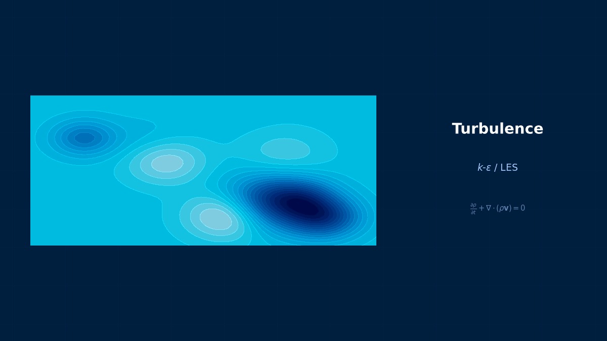
LES (Large Eddy Simulation) Explained
Professor, I heard that LES is a method somewhere between RANS and DNS. What exactly is the underlying concept?
Good question. Turbulence contains eddies of various scales. LES uses spatial filtering to directly calculate the large-scale eddies, while the eddies smaller than the filter width (subgrid-scale, SGS) are approximated by a model.
I see, so you directly solve for the large eddies and only model the small ones. How does it differ from DNS?
DNS resolves all eddies down to the Kolmogorov scale $\eta_K$, requiring grid points on the order of $N \sim Re^{9/4}$. This is completely infeasible for industrial problems at practical Reynolds numbers. LES significantly reduces computational cost by taking the filter width $\Delta$ larger than the Kolmogorov scale.
Mathematical Definition of Spatial Filtering
What exactly is the mathematical operation for "filtering"?
For any physical quantity $\phi(\mathbf{x}, t)$, the filter operation is defined by a convolution integral.
$$ \bar{\phi}(\mathbf{x}, t) = \int_{-\infty}^{\infty} G(\mathbf{x} - \mathbf{x}', \Delta) \, \phi(\mathbf{x}', t) \, d\mathbf{x}' $$
Here, $G$ is the filter kernel, and $\Delta$ is the filter width. Typical filters include the Box (top-hat) filter, Gaussian filter, and Sharp spectral (cut-off) filter.
Which filter is actually used in CFD codes?
In finite volume method-based codes (Fluent, STAR-CCM+, OpenFOAM, etc.), implicit filtering based on cell volume is common. The filter width is often defined as the cell characteristic length, such as $\Delta = V_{cell}^{1/3}$ or $\Delta = (\Delta x \cdot \Delta y \cdot \Delta z)^{1/3}$.
Filtered Navier-Stokes Equations
What happens when you apply filtering to the Navier-Stokes equations?
For incompressible flow, the filtered continuity and momentum equations become:
$$ \frac{\partial \bar{u}_i}{\partial x_i} = 0 $$
$$ \frac{\partial \bar{u}_i}{\partial t} + \frac{\partial (\bar{u}_i \bar{u}_j)}{\partial x_j} = -\frac{1}{\rho}\frac{\partial \bar{p}}{\partial x_i} + \nu \frac{\partial^2 \bar{u}_i}{\partial x_j \partial x_j} - \frac{\partial \tau_{ij}^{sgs}}{\partial x_j} $$
The key point here is that the nonlinear term $\overline{u_i u_j}$ cannot be approximated by the product of filtered velocities $\bar{u}_i \bar{u}_j$, giving rise to the SGS stress tensor.
$$ \tau_{ij}^{sgs} = \overline{u_i u_j} - \bar{u}_i \bar{u}_j $$
So this $\tau_{ij}^{sgs}$ is what needs to be modeled, right?
Exactly. The models used to close the SGS stress tensor are called SGS models (subgrid-scale models). Various models have been proposed, such as the Smagorinsky model, dynamic Smagorinsky model, and WALE model.
Eddy Viscosity Hypothesis
Many SGS models seem to use the concept of "eddy viscosity". What is that?
It applies the Boussinesq hypothesis to the small-scale eddies, making the deviatoric component of the SGS stress tensor proportional to the strain rate tensor.
$$ \tau_{ij}^{sgs} - \frac{1}{3}\tau_{kk}^{sgs}\delta_{ij} = -2\nu_{sgs}\bar{S}_{ij} $$
Here, $\bar{S}_{ij} = \frac{1}{2}\left(\frac{\partial \bar{u}_i}{\partial x_j} + \frac{\partial \bar{u}_j}{\partial x_i}\right)$ is the filtered strain rate tensor, and $\nu_{sgs}$ is the SGS eddy viscosity coefficient. The difference between SGS models lies in how they evaluate this $\nu_{sgs}$.
It's a similar concept to RANS eddy viscosity. But the difference is that in LES it's calculated as a local, instantaneous value, right?
Exactly. RANS uses a time-averaged eddy viscosity, while LES evaluates a local eddy viscosity for the instantaneous filtered field. This difference is physically very significant.
Coffee Break Trivia
The Origin of the Name "Filter"
The concept of "spatial filtering" in LES was first systematized by meteorologist Joseph Smagorinsky. The idea in his 1963 paper was simple: "Let's solve only the large-scale atmospheric motions and parameterize the effects of small-scale turbulence by averaging them." The term "filter width $\Delta$," now commonplace in CFD, also originates from the grid spacing of weather models. It's quite an interesting journey that an idea from wind forecasting models is now being repurposed for engine combustion simulations, isn't it?
Professor, I heard that LES is a method somewhere between RANS and DNS. What exactly is the underlying concept?
Good question. Turbulence contains eddies of various scales. LES uses spatial filtering to directly calculate the large-scale eddies, while the eddies smaller than the filter width (subgrid-scale, SGS) are approximated by a model.
I see, so you directly solve for the large eddies and only model the small ones. How does it differ from DNS?
DNS resolves all eddies down to the Kolmogorov scale $\eta_K$, requiring grid points on the order of $N \sim Re^{9/4}$. This is completely infeasible for industrial problems at practical Reynolds numbers. LES significantly reduces computational cost by taking the filter width $\Delta$ larger than the Kolmogorov scale.
What exactly is the mathematical operation for "filtering"?
For any physical quantity $\phi(\mathbf{x}, t)$, the filter operation is defined by a convolution integral.
Here, $G$ is the filter kernel, and $\Delta$ is the filter width. Typical filters include the Box (top-hat) filter, Gaussian filter, and Sharp spectral (cut-off) filter.
Which filter is actually used in CFD codes?
In finite volume method-based codes (Fluent, STAR-CCM+, OpenFOAM, etc.), implicit filtering based on cell volume is common. The filter width is often defined as the cell characteristic length, such as $\Delta = V_{cell}^{1/3}$ or $\Delta = (\Delta x \cdot \Delta y \cdot \Delta z)^{1/3}$.
What happens when you apply filtering to the Navier-Stokes equations?
For incompressible flow, the filtered continuity and momentum equations become:
The key point here is that the nonlinear term $\overline{u_i u_j}$ cannot be approximated by the product of filtered velocities $\bar{u}_i \bar{u}_j$, giving rise to the SGS stress tensor.
So this $\tau_{ij}^{sgs}$ is what needs to be modeled, right?
Exactly. The models used to close the SGS stress tensor are called SGS models (subgrid-scale models). Various models have been proposed, such as the Smagorinsky model, dynamic Smagorinsky model, and WALE model.
Many SGS models seem to use the concept of "eddy viscosity". What is that?
It applies the Boussinesq hypothesis to the small-scale eddies, making the deviatoric component of the SGS stress tensor proportional to the strain rate tensor.
Here, $\bar{S}_{ij} = \frac{1}{2}\left(\frac{\partial \bar{u}_i}{\partial x_j} + \frac{\partial \bar{u}_j}{\partial x_i}\right)$ is the filtered strain rate tensor, and $\nu_{sgs}$ is the SGS eddy viscosity coefficient. The difference between SGS models lies in how they evaluate this $\nu_{sgs}$.
It's a similar concept to RANS eddy viscosity. But the difference is that in LES it's calculated as a local, instantaneous value, right?
Exactly. RANS uses a time-averaged eddy viscosity, while LES evaluates a local eddy viscosity for the instantaneous filtered field. This difference is physically very significant.
The Origin of the Name "Filter"
The concept of "spatial filtering" in LES was first systematized by meteorologist Joseph Smagorinsky. The idea in his 1963 paper was simple: "Let's solve only the large-scale atmospheric motions and parameterize the effects of small-scale turbulence by averaging them." The term "filter width $\Delta$," now commonplace in CFD, also originates from the grid spacing of weather models. It's quite an interesting journey that an idea from wind forecasting models is now being repurposed for engine combustion simulations, isn't it?
Computational Methods for LES Fundamentals
Spatial Discretization for LES
When implementing LES, what should I be careful about regarding spatial discretization?
LES requires accurately resolving eddy structures at scales larger than the filter width, so schemes with low numerical dissipation are needed. Second-order central differencing is the minimum baseline; ideally, higher-order central differencing or compact differencing should be used.
Is upwind differencing no good?
First-order upwind differencing must absolutely not be used. Its numerical dissipation far exceeds the dissipation from the SGS model, artificially wiping out eddy structures. Even second-order upwind requires caution; when using blending schemes (e.g., a mix of central and upwind differencing), the proportion of central differencing should be sufficiently high. OpenFOAM's linearUpwind or Fluent's Bounded Central Differencing are practical compromises, but if the central differencing proportion is too low, LES loses its meaning.
Time Integration Schemes
How should time be discretized?
Since LES is inherently an unsteady calculation, time integration accuracy is also important. At least second-order accuracy is required. Typical choices are as follows:
| Scheme | Accuracy | Features |
|---|---|---|
| 2nd-order Backward Difference (BDF2) | 2nd | Implicit, stable, OpenFOAM's 'backward' |
| Crank-Nicolson | 2nd | Implicit, can be oscillatory |
| Adams-Bashforth 2nd order | 2nd | Explicit, has CFL restriction |
| Runge-Kutta 3rd/4th order | 3rd-4th | Explicit, high accuracy, common in spectral codes |
Are there any guidelines for determining the time step size?
Manage it using the CFL number (Courant-Friedrichs-Lewy number). For explicit schemes, $CFL < 1$ is the stability condition, but even for implicit schemes, it's desirable to keep $CFL \sim 1$ to ensure LES accuracy. The CFL number is defined as $CFL = \frac{u \Delta t}{\Delta x}$.
Pressure-Velocity Coupling
How is pressure-velocity coupling handled for incompressible LES?
The PISO (Pressure Implicit with Splitting of Operators) method is the most common. Within each time step, it performs one predictor step and two or more corrector steps. In OpenFOAM, the pimpleFoam solver adopts the PIMPLE (PISO+SIMPLE) algorithm and is widely used for LES. In Fluent, the combination of Non-Iterative Time Advancement (NITA) + fractional step method is recommended.
Grid Resolution Requirements
How fine does the mesh need to be for LES? It seems completely different from RANS.
For wall-resolved LES (wall-resolved LES, WRLES), the grid resolution near the wall has very stringent requirements.
| Direction | Requirement (wall units) | Notes |
|---|---|---|
| Wall-normal direction $\Delta y^+$ | < 1 (first cell) | Resolve viscous sublayer |
| Streamwise direction $\Delta x^+$ | 50 - 100 | Resolve streak structures |
| Spanwise direction $\Delta z^+$ | 15 - 40 | Resolve streamwise vortices |
Here, wall units are $y^+ = y u_\tau / \nu$, $u_\tau = \sqrt{\tau_w/\rho}$.
It has to be that fine? The computational cost seems enormous.
Exactly. The number of grid points for wall-resolved LES increases on the order of $N \sim Re^{13/7}$, making it extremely costly for real-world problems at high Reynolds numbers. That's why hybrid methods like wall-modeled LES (WMLES) and DES/IDDES become important.
The Long Battle with LES's "Numerical Viscosity"
When choosing a discretization scheme for LES, why go to the trouble of using second-order accuracy...
Related Topics
Experience the theory firsthand with the interactive simulator for this field
All Simulators