Thermal Simulation of Thermal Storage Materials (PCM)
Thermal Simulation of Thermal Storage Materials: Theoretical Foundations
What is PCM?
Professor, PCM is a thermal storage material, right? What exactly do we solve in the simulation?
Good question. PCM (Phase Change Material) is a material that absorbs a large amount of heat when it changes from solid to liquid—that is, when it melts. The essence of thermal storage is using this "latent heat" to control temperature.
Controlling temperature with latent heat...? Could you explain a bit more concretely!
For example, when ice melts at 0°C, it absorbs 334 kJ/kg of heat without its temperature rising, right? PCM utilizes this principle. Paraffin-based PCMs have a latent heat of about 200 kJ/kg near a melting point of 28°C, and salt hydrates have about 260 kJ/kg near 32°C. Designs that fill the spaces between cells with PCM to keep battery pack temperatures below 40°C have been rapidly increasing in recent years.
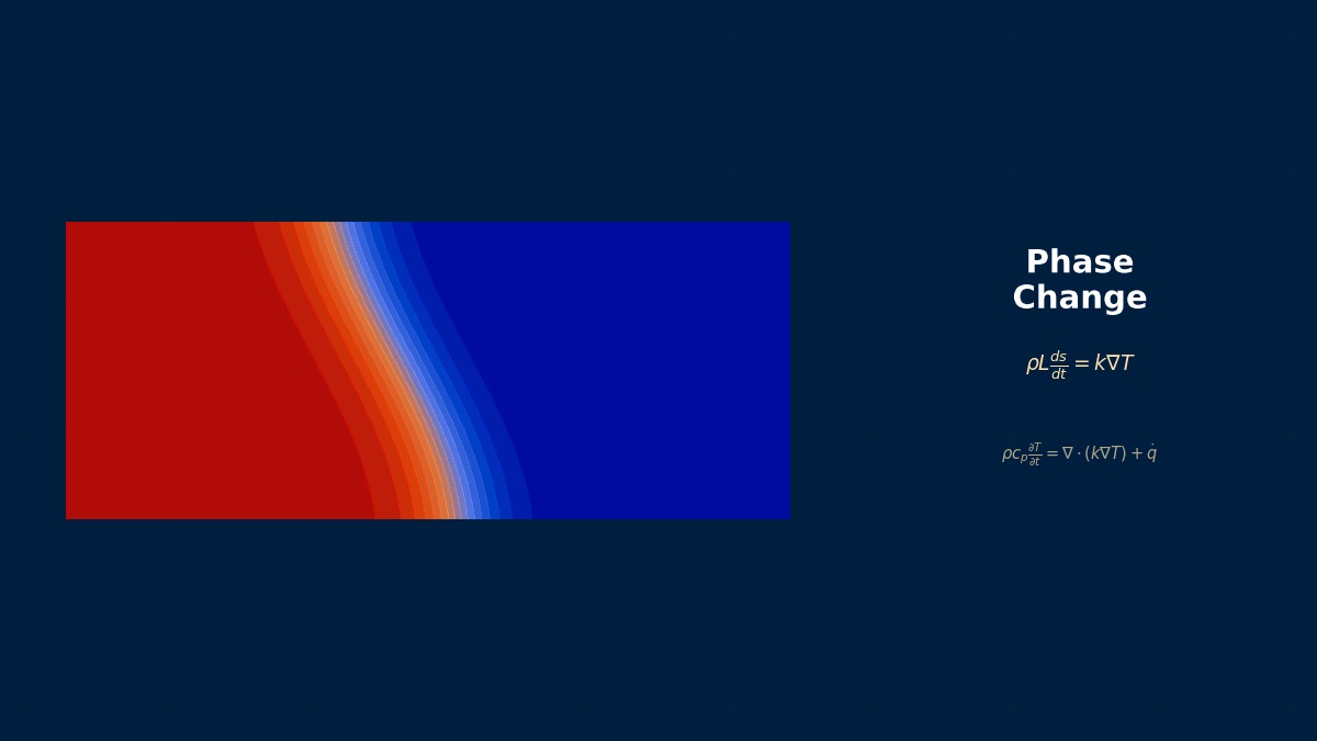
I see, so while it's melting, the temperature doesn't rise, acting like a "temperature wall"! And what we solve in the simulation is...?
Predicting how the solid-liquid boundary—the melting front—moves, when and how far it melts, and how the temperature rises after it's completely melted. This is a classic moving boundary problem called the "Stefan problem." In CAE, the mainstream approach is to solve it using the enthalpy method without explicitly tracking the boundary.
Stefan Problem and Moving Boundary
I've heard the name Stefan problem before. It's the problem where the melting part moves, right?
That's right. Let's consider a one-dimensional Stefan problem. Suppose there is a PCM slab heated to a high temperature on one side. If the position of the solid-liquid interface is $s(t)$, then at the interface, the condition "the interface advances while absorbing latent heat" holds:
Here, $L$ is the latent heat per unit mass [J/kg], $k_s, k_l$ are the thermal conductivities of the solid and liquid phases respectively, and $T_s, T_l$ are the temperature fields of the solid and liquid phases. The difference in heat flux from both sides of the interface becomes the energy source for melting.
Tracking the interface seems tough... you'd have to move the mesh too, right?
Exactly. That's why in practice, the enthalpy method, which avoids interface tracking, is used most of the time. The idea is "we don't need to know where the interface is; as long as the energy balance is correct, the temperature field will come out right."
Governing Equations of the Enthalpy Method
Please show me the equations for the enthalpy method!
In the enthalpy method, we solve the energy conservation equation with enthalpy per unit volume $H(T)$ as the variable:
Here, the enthalpy $H(T)$ is defined as a function of temperature as follows:
Here, $f_l(T)$ is the liquid fraction, a function that varies from $0$ (completely solid) to $1$ (completely liquid). $\epsilon$ is the half-width of the mushy zone; for pure substances $\epsilon \to 0$, while for alloys or paraffin mixtures it is on the order of a few °C.
If I imagine the graph of $H(T)$, does it jump suddenly at the melting point?
Correct! For pure substances, it jumps vertically at the melting point. For materials with a melting temperature range like paraffins or salt hydrates, it becomes a sloped step. The height of this jump corresponds to the latent heat $L$. In simulation, this sharp change causes nonlinearity, so care is needed with time steps and mesh.
Apparent Heat Capacity Method
Are there other methods besides the enthalpy method?
Another well-known method is the Apparent Heat Capacity Method. It models latent heat as an apparent specific heat $c_{p,eff}$ over the melting temperature range:
In implementation, the Dirac delta function $\delta$ is approximated by a Gaussian distribution or hat function, expressed as a peak with width $2\epsilon$:
Which is better, the enthalpy method or the apparent heat capacity method?
Practically, the enthalpy method is overwhelmingly advantageous. With the apparent heat capacity method, if the time step is coarse, it can skip over the melting temperature range entirely and miss the latent heat—this is the so-called "latent heat skip". The phase change modules in Ansys Fluent and COMSOL internally use the enthalpy method; the apparent heat capacity method is a simplified technique when reusing a standard FEM thermal analysis solver.
| Characteristic | Enthalpy Method | Apparent Heat Capacity Method |
|---|---|---|
| Energy Conservation | ◎ Strictly conserved | △ Time step dependent |
| Latent Heat Skip Risk | None | Present (occurs with large $\Delta t$) |
| Ease of Implementation | ○ Requires dedicated module | ◎ Can be used with standard thermal analysis |
| Mushy Zone Representation | Can be represented naturally | Choice of $\epsilon$ is critical |
| Main Adopting Solvers | Fluent, STAR-CCM+, COMSOL | Abaqus, Nastran (via UDL) |
Physical Meaning of the Stefan Number Ste
What is the Stefan number? How is it used?
The Stefan number is a dimensionless number representing the ratio of sensible heat to latent heat. It serves as an indicator to quantify the "difficulty" of PCM simulation:
Here, $\Delta T$ is the degree of superheat (e.g., the difference between wall temperature and melting point $T_{wall} - T_m$), and $L$ is the latent heat.
What changes when Ste is large?
Roughly speaking:
- $\mathrm{Ste} \ll 1$ (Latent heat dominant): Melting progresses slowly. PCM cooling for battery packs is in this region. If $\Delta T = 12$°C, $c_p = 2000$ J/(kg·K), $L = 200{,}000$ J/kg, then $\mathrm{Ste} = 0.12$. Time steps can be relatively large.
- $\mathrm{Ste} \gg 1$ (Sensible heat dominant): Almost like a normal heat conduction problem. Solidification in casting (hundreds of °C $\Delta T$) is an example. Time steps need to be fine to avoid numerical oscillation.
- $\mathrm{Ste} \sim 0.1$: The region where Neumann's approximate solution can be used. The melting front position can be estimated as $s(t) \approx 2\lambda\sqrt{\alpha t}$, which is convenient for verifying analysis results.
Types of PCM Materials and Property Values
Are there other PCM materials besides paraffin?
They are broadly classified into three types. Let's organize them along with the property values needed for simulation:
| PCM Type | Representative Materials | Melting Point [°C] | Latent Heat [kJ/kg] | $k$ [W/(m·K)] | Applications |
|---|---|---|---|---|---|
| Organic (Paraffin) | RT28HC, n-Octadecane | 24~32 | 180~250 | 0.2 | Battery cooling, building |
| Inorganic (Salt Hydrate) | CaCl₂·6H₂O, Na₂SO₄·10H₂O | 29~32 | 170~265 | 0.5~1.1 | Floor heating, cold storage |
| Eutectic | Organic+Organic, Organic+Inorganic mixtures | Design freedom | 120~200 | 0.2~0.8 | Design for specific temperature ranges |
| Metallic | Ga, Bi-Sn alloy | 30~140 | 60~80 | 20~40 | High heat flux electronics |
Paraffin's thermal conductivity is 0.2... that's incredibly low...
Yes, this is the biggest practical challenge in PCM simulation. Low thermal conductivity makes the melting rate extremely slow. So in actual products, aluminum fins are added or carbon nanotubes are dispersed to increase the effective thermal conductivity. In simulation, you either treat it as a composite of "PCM + fins" or use homogenized effective property values—this is where the designer's skill comes in.
NASA's PCM Temperature Control
NASA has used PCM for temperature control of space equipment since the Apollo program in the 1960s. On the lunar surface, with its harsh temperature environment of +127°C in sunlight / -173°C in shadow, the electronic equipment housing of the lunar rover equipped with paraffin-based PCM maintained internal temperatures between -20°C and +50°C. Improved PCM modules are also installed on the 2020s Mars rover Perseverance. Coupled analysis including radiative heat transfer in a vacuum is essential for simulation, which is exactly where CAE comes in.
Computational Methods for Thermal Simulation of Thermal Storage Materials
Spatial Discretization and Time Integration
How do we solve the enthalpy method on a computer?
With FVM (Finite Volume Method), you can directly treat the enthalpy per cell as a conserved quantity, so it's a good match. Ansys Fluent and STAR-CCM+ use this approach. With FEM (Finite Element Method), it's discretized after converting to the weak form.
Here is the discretized equation based on FVM. Discretizing the energy conservation equation for cell $i$ implicitly gives:
Here, $V_i$ is the cell volume, $A_f$ is the face area, $\delta_f$ is the distance between cell centers, and the subscript $nb$ denotes the neighboring cell. Since there is an $H(T)$ relationship between $H_i^{n+1}$ and $T_i^{n+1}$, it is solved iteratively using Newton's method or source-based linearization.
For time integration, which is better, implicit or explicit methods?
For PCM, implicit methods (backward Euler) are the iron rule. There are two reasons:
- Paraffin has low thermal conductivity, so to satisfy the stability condition $\mathrm{Fo} = \alpha \Delta t / \Delta x^2 \leq 0.5$, a very small time step is required.
- The sharp change in enthalpy (latent heat jump) creates strong nonlinearity, but with implicit methods, you can iterate to convergence at each time step.
Handling the Mushy Zone
I often hear "mushy zone"—what is it?
It's the intermediate state—neither solid nor liquid—where solid and liquid coexist. For paraffin mixtures, the melting point spreads over a range like 28~32°C, so that entire temperature band becomes the mushy zone.
In Ansys Fluent's Solidification/Melting model, the liquid fraction $f_l$ in the mushy zone is linearly interpolated as follows:
Furthermore, to suppress flow in the mushy zone, a Darcy-type source term (Enthalpy-Porosity method) is added to the momentum equation:
Here, $C_{mush}$ is the mushy zone constant (typical values $10^5$ to $10^8$), and $\varepsilon_{mush}$ is a small constant to prevent division by zero (usually $10^{-3}$). The behavior is such that $f_l \to 0$ (solid) gives $S \to \infty$ (completely stops flow), and $f_l \to 1$ (liquid) gives $S \to 0$ (flow freely).
How do you decide the value of $C_{mush}$? $10^5$ and $10^8$ are completely different...
Actually, selecting $C_{mush}$ is the "artisan" part of PCM simulation. For pure paraffin, $10^5$ to $10^6$ is common, adjusted to match experimental melting front positions. If $C_{mush}$ is too large, the mushy zone becomes too stiff and melting slows down; if it's too small, unphysical flow occurs in the solid region. Papers always perform a "$C_{mush}$ sensitivity analysis," so I recommend trying at least three levels.
Modeling Natural Convection in the Liquid Phase
Does the melted liquid move? Isn't heat conduction alone enough?
It moves a lot. This is the tricky part of PCM simulation. Melted paraffin develops density differences due to temperature differences, causing buoyancy-driven natural convection. When the Rayleigh number exceeds $10^5$, convective effects become dominant, and melting can progress 2~5 times faster than predicted by pure conduction.
Using the Boussinesq approximation:
Related Topics
Experience the theory with interactive simulators in this field
PCM Melting Simulator Thermal Analysis Tools List