NovaSolver›Monte Carlo Radiative Transfer (MCRT) Simulator Back
Computational Radiative Transfer
Monte Carlo Radiative Transfer (MCRT) Simulator
Track individual photons random-walking through an absorbing and scattering slab and read the diffuse reflectance, transmittance and penetration depth in real time. The MCML-style framework you see here is shared by tissue optics, photodynamic therapy, thin-film optics and interstellar-dust radiative transfer alike.
Parameters
Absorption coefficient μ_a
1/cm
Per-cm absorption probability. 0.01–1 typical for tissue
Scattering coefficient μ_s
1/cm
Scattering events per cm. 10–500/cm for tissue
Anisotropy g
Henyey-Greenstein. g=0 isotropic, g→1 forward
Slab thickness d
mm
Photon count log₁₀(N)
Tracked photons. N = 10^value, error scales as 1/√N
Refractive index n
Refractive index of the medium. 1.37–1.45 for tissue
Wavelength λ
nm
Incident wavelength. Visible to near-infrared
Results
—
Mean free path ℓ (cm)
—
Transport MFP ℓ* (cm)
—
Optical depth τ'
—
Diffuse reflectance R (%)
—
Diffuse transmittance T (%)
—
Penetration depth δ_p (mm)
—
Photon random walk — MCRT animation
Photons (white) entering the slab from above are scattered (blue), absorbed (red), reflected (green) or transmitted (orange). Colour shows the terminal mode of each photon.
Reflectance R / Transmittance T vs optical depth τ'
Penetration depth δ_p vs absorption/scattering ratio μ_a/μ_s
$$p_{HG}(\cos\theta) = \frac{1}{4\pi}\,\frac{1-g^2}{(1+g^2 - 2g\cos\theta)^{3/2}},\qquad s = -\frac{\ln(\xi)}{\mu_t}$$
Henyey-Greenstein phase function and sampled free path s. ξ ∈ (0,1] is a uniform random number.
Monte Carlo Radiative Transfer — Photon Tracking in Absorbing/Scattering Media
🙋
"Monte Carlo radiative transfer" — is that the method that computes how a laser beam spreads inside a medium? Why does it need random numbers?
🎓
Exactly. The radiative transfer equation (RTE) for a medium that scatters and absorbs is a 7-dimensional integro-differential equation, essentially unsolvable analytically. So MCRT just says, "let's chase one photon at a time with dice rolls." Per photon you only need three rules: (1) sample the free path from an exponential distribution, (2) sample the scattering angle from the phase function, (3) decide absorb-or-scatter via the albedo. Run millions of photons and you reconstruct the RTE solution.
🙋
Brute force but conceptually clean. When I sweep "Anisotropy g" from 0 to 0.9 the transport MFP ℓ* jumps. What's going on?
🎓
g measures the forward bias of scattering: g=0 is fully isotropic, g→1 is pure forward scattering. In tissue g≈0.9, meaning an average scattering event deflects the photon by only ~25°. The photon needs many scatterings to forget its initial direction, and the cumulative distance for that is ℓ* = 1/(μ_a + (1-g)μ_s). Switching g from 0 to 0.9 multiplies ℓ* by ~10. "Light goes deep but also spreads quickly" is exactly this effect.
🙋
δ_p = 17.4 mm sounds deep. Does red light really reach that far into skin?
🎓
The defaults μ_a=0.1, μ_s=10 are a weak-absorption, strong-scattering example and let light travel a bit more than real skin (μ_a≈0.3–2/cm), which gives δ_p of a few millimetres in vivo. Even so, 670 nm red still reaches deep dermis, which is why low-level laser therapy (LLLT) and photodynamic therapy (PDT) use it. Different wavelengths change μ_a and μ_s drastically, so in clinical work you pick the wavelength based on the target depth.
🙋
Raising N drops the statistical error. So why is MCRT considered slow?
🎓
Because the error only falls as 1/√N — that's the bottleneck. To cut the error by 10, you need 100× more photons. Standard MCML costs tens of microseconds per photon, so N=10⁶ takes tens of seconds to minutes; 3D heterogeneous models cost much more. That's why people invest in (1) GPU parallelism, (2) variance reduction (Russian roulette, photon splitting), and (3) importance sampling. CUDA-MCML or MCX can push billions of photons per second.
🙋
Is MCRT used outside biomedical optics too?
🎓
MCRT is really a cross-disciplinary meta-method. Interstellar dust radiative transfer (DUSTY / HYPERION), combustion radiation in CFD, light trapping in solar cells, OLED and thin-film optics, PET/SPECT calibration, ocean optics — anywhere scattering and absorption coexist, MCRT applies. Neutron transport (MCNP) uses the same recipe and is the workhorse for nuclear reactor design. The physical kernel changes; the sampling structure does not.
Frequently Asked Questions
MCRT solves the radiative transfer equation (RTE) by tracking individual photons one by one using probabilistic models instead of an analytical approach. The free path to the next scattering or absorption event is sampled from an exponential distribution with mean 1/(μ_a + μ_s), the scattering angle from the Henyey-Greenstein phase function with anisotropy g, and the absorb-or-scatter decision from the single-scattering albedo a = μ_s/(μ_a + μ_s). Averaging over many photons recovers the RTE solution. The MCML code by Wang, Jacques and Zheng is the de facto standard in tissue optics.
The mean free path ℓ = 1/(μ_a + μ_s) is the average distance the photon travels in a straight line before the next event. The transport mean free path ℓ* = 1/(μ_a + μ_s') is the distance over which the photon loses memory of its initial direction, using the reduced scattering coefficient μ_s' = (1-g)·μ_s. For strongly forward-peaked scattering (g→1), one event barely changes the direction, so ℓ* ≫ ℓ and the medium effectively looks "thicker". In tissue with g ≈ 0.9, ℓ* is about 10× ℓ. The diffusion approximation is built on ℓ*.
δ_p = 1/√(3 μ_a (μ_a + μ_s')) is the depth at which the diffuse fluence decays to 1/e inside a scattering medium. In a semi-infinite medium the internal fluence roughly follows exp(-z/δ_p). For laser therapy and photodynamic therapy (PDT), δ_p controls how deep the drug activates, and the wavelength is chosen to tune δ_p. For 670 nm red light in skin, δ_p is on the order of a few millimetres.
Monte Carlo averages over N independent photon histories, and by the central limit theorem the standard error of the estimate falls as 1/√N. That gives 1% error at N=10⁴ and 0.1% error at N=10⁶. Cutting the error by a factor of 10 takes 100× more photons, which is MCRT's main weakness. In practice, variance reduction (Russian roulette, photon splitting, importance sampling) and GPU parallelism are used to bring runtimes down.
Real-World Applications
Tissue optics and photodynamic therapy (PDT): For PDT of skin cancers, oesophageal lesions and AMD in the eye, a photosensitiser (PpIX, verteporfin, etc.) is concentrated in tissue and illuminated with laser light; reactive oxygen species destroy the diseased cells. Treatment depth is governed by "how far the light goes", so MCML-class MCRT is run beforehand to estimate δ_p and pick the wavelength (green 532 nm vs red 630 nm vs near-infrared 800 nm) and dose. This is the standard simulation method in dermatology photonics and ophthalmology.
Nuclear imaging and diffuse optical tomography (PET/SPECT/DOT): Detector response of PET/SPECT and image reconstruction for diffuse optical tomography (DOT) and fNIRS use MCRT outputs (sensitivity matrices) as the forward problem. fNIRS brain imaging runs multilayer scalp–skull–brain MCRT to visualize "which depths the signal samples", separating noise (scalp blood flow) from cortical activity.
CFD combustion radiation and astrophysics: Furnace radiation in gas-turbine combustors, boilers and rocket engines includes scattering and absorption from soot and gas, so it is computed by CFD-coupled MCRT. Alongside Fluent's DTRM/Discrete Ordinates, Photon Monte Carlo is the high-accuracy reference. In astrophysics, radiative transfer in dust discs and circumstellar envelopes (DUSTY / HYPERION / RADMC-3D) is the workhorse, allowing direct comparison between modelled and observed spectra.
Photovoltaics, thin-film optics and OLED design: Light harvesting and extraction in textured Si solar cells, perovskite films and multilayer OLEDs are evaluated by combining wave-optical FDTD with geometric-optical MCRT. MCRT is the right tool when reflectors and textures dominate, and it is used in Sunpower and tandem-cell optimisation.
Common Misconceptions and Pitfalls
The first pitfall is assuming "more photons N always wipes out the error". The MCRT error only falls as 1/√N. With N = 10⁵ this tool reports ~0.32% error, but that is the error on a global average. Local quantities (such as depth-resolved absorption profiles) carry larger error, easily exceeding 10% in deep or weakly absorbing regions where few photons arrive. Producing accurate depth profiles requires variance reduction (Russian roulette, photon splitting, bias scattering).
Second, the diffusion approximation and MCRT are not the same thing. The analytic R and T expressions in this tool come from δ_p and semi-infinite-slab approximations and only hold when scattering dominates absorption (μ_s' ≫ μ_a) and when the slab is much thicker than ℓ. Within one ℓ of the surface, in strongly absorbing regions (melanin, blood vessels) or near interfaces, the diffusion approximation breaks down. Research-grade design always runs full MCML; the diffusion approximation stays as a back-of-the-envelope tool.
Finally, the Henyey-Greenstein phase function is not perfect. HG is a convenient one-parameter approximation to Mie scattering, but its back-scattering and ~90° behaviour can be off by tens of per cent. For systems where back-scattering matters (e.g. skin), the Modified HG (Reynolds-McCormick) function or a tabulated Mie phase function gives better accuracy. In academic tissue optics, two-term models (g₁, g₂) or measured wavelength-dependent g(λ) are the norm rather than a single g.
How to Use
Set absorption coefficient (μa, cm⁻¹) and scattering coefficient (μs, cm⁻¹) for your tissue or material type—typical skin: μa=0.1–0.5, μs=10–50
Adjust anisotropy factor g (0–1, where g=0 is isotropic scattering, g≈0.9 for forward-peaked biological tissue)
Specify slab thickness (mm) and number of photon packets to launch; simulator tracks each photon's random walk until absorption or boundary exit
Run simulation and record diffuse reflectance R, transmittance T, mean free path ℓ, and penetration depth δ_p from output statistics
Worked Example
For 1 mm thick human dermis with μa=0.15 cm⁻¹, μs=30 cm⁻¹, g=0.85: mean free path ℓ=333 μm, transport MFP ℓ*=1.67 mm, optical depth τ'=3.0. Running 100,000 photon packets yields diffuse reflectance R≈32%, transmittance T≈18%, penetration depth δ_p≈0.6 mm. Increasing μs to 50 cm⁻¹ reduces ℓ to 200 μm and increases R to 48% due to stronger backscattering.
Practical Notes
Convergence: use ≥50,000 photons for smooth reflectance/transmittance curves; noisy statistics below 10,000 packets indicate insufficient sampling
Biological validation: compare outputs against literature (e.g., porcine skin μs≈40, R~30–40%) or measured diffuse reflectance spectra
Scattering dominance: when μs≫μa, photons scatter many times before exit; when μa≫μs, absorption dominates and transmittance drops sharply
Parameter sensitivity: doubling g shifts R by ~5–10%; g-dependent transport MFP ℓ*=ℓ/(1−g) is critical for dose estimation in optical therapy
🎬 Watch it in motion
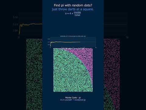
Monte Carlo | a rain of random dots pins down pi #Shorts