NovaSolver›Quasi-Monte Carlo Simulator — Sobol Sequence Back
Numerical Methods
Quasi-Monte Carlo Simulator — Sobol Sequence
Integrate numerically with low-discrepancy sequences such as the Sobol and Halton sequences. Change the sample count, sequence type and integrand to watch how deterministic point sets fill the unit square evenly and converge far faster than pseudo-random sampling.
Parameters
Sample count N
Number of points placed in the unit square
Sequence type
How the points are placed
Integrand
Function integrated over the unit square [0,1]²
Results
—
Integral estimate
—
True value
—
Absolute error
—
Sequence type
—
Accuracy gain vs random
—
Sample count
—
Point placement on the unit square
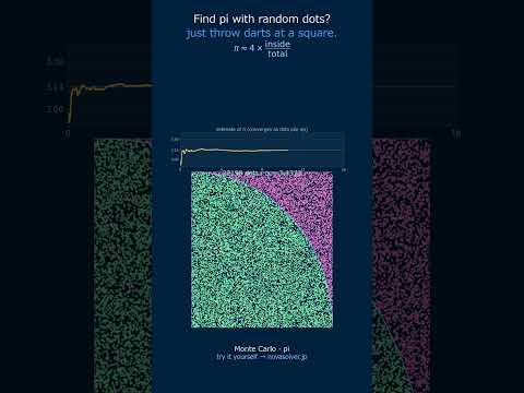
Sample points placed in the unit square [0,1]². Pseudo-random points clump and leave gaps; Sobol and Halton points spread out evenly. For the circle integrand the points inside the arc are coloured differently.
Numerical integration approximates the integral by the average of the integrand f evaluated at the sample points x_i. The choice of point set decides the speed of convergence.
Pseudo-random Monte Carlo converges only as 1/√N, but a low-discrepancy sequence fills the domain evenly, so the quasi-Monte Carlo error converges much faster (d is the dimension).
The Koksma–Hlawka inequality. The integration error is bounded by the product of the function's total variation V(f) and the point set's star discrepancy D*_N.
What is the Quasi-Monte Carlo Simulator?
🙋
How is "quasi-Monte Carlo" different from ordinary Monte Carlo? The names are so similar that I can't tell them apart.
🎓
Good question. Ordinary Monte Carlo integration scatters points with "random numbers" — like rolling dice — and estimates the integral as the average of the function values at those points. It is convenient, but random numbers are actually uneven. Set the sequence on the left to "Pseudo-random" and look at the canvas. The points clump together like dumplings in some places and leave gaps in others, right? Quasi-Monte Carlo deliberately replaces those random points with a fixed point set designed to spread out evenly.
🙋
You'd think random points would scatter "fairly", but they clump up. When I switch to the Sobol sequence the points line up neatly, almost like a grid.
🎓
Yes, that is the counter-intuitive part. Random numbers decide "where to put the next point" independently of the past points, so nothing stops two points from landing close together — hence the clumps. Sobol and Halton sequences are called "low-discrepancy sequences": they fill the space without gaps at every scale, avoiding the points already placed. Integration lives or dies on "how evenly you sampled points that represent the domain", so that uniformity translates directly into accuracy.
🙋
The word "discrepancy" came up — what exactly does it measure?
🎓
Roughly speaking, it measures "how biased the points are". Take any box of any size inside the domain. Ideally the fraction of points inside that box matches the box's area exactly. Discrepancy is the worst such mismatch over all boxes. Pseudo-random points have clumps, so the mismatch is large; Sobol points keep it small. The Koksma–Hlawka inequality tells us "integration error ≤ function variation × discrepancy". So if you make the discrepancy small, you also push down the error bound.
🙋
In the "Error convergence" chart below, the Sobol line drops more steeply. Is that the effect you mean?
🎓
Exactly. On a log-log chart the slope shows the speed of convergence. The pseudo-random error is 1/√N — quadruple the points just to halve the error. Quasi-Monte Carlo is close to (log N)ᵈ/N, almost 1/N — quadruple the points and the error drops to nearly a quarter. For the same accuracy you need orders of magnitude fewer samples. That is why "the Sobol sequence is the default" for option pricing in computational finance and for rendering.
🙋
So should I always use the Sobol sequence? Are there no drawbacks?
🎓
It is not a cure-all. Notice the (log N)ᵈ term in the error bound. When the dimension d is very large, that power of the logarithm starts to bite and the advantage fades. And if the integrand is discontinuous or has infinite total variation, the Koksma–Hlawka guarantee no longer holds. In practice engineers "scramble" the Sobol sequence with a small random shift, getting both the good determinism and an easy error estimate. Start by using this tool to feel the difference in convergence as you switch sequences.
Frequently Asked Questions
Ordinary Monte Carlo integration scatters pseudo-random points, so they clump together in some places and leave gaps in others, and the error falls only as 1/√N. Quasi-Monte Carlo replaces the random points with a deterministic low-discrepancy sequence such as the Sobol or Halton sequence, carefully constructed to fill the domain as uniformly as possible at every scale. Because the coverage is so even, the error falls almost as fast as (log N)ᵈ/N, so the same accuracy is reached with dramatically fewer samples.
Discrepancy measures how evenly a point set fills the space. For any small box inside the domain, you compare the fraction of points that fall inside the box with the box's volume (area); discrepancy is the worst such mismatch over all boxes. Pseudo-random points have clumps and gaps, so their discrepancy is large; Sobol and Halton sequences are built specifically to keep it small. The Koksma–Hlawka inequality bounds the integration error by the product of the function's total variation and the point set's discrepancy.
A Sobol sequence prepares a set of integer 'direction numbers' for each dimension and generates each point by XOR-accumulating direction numbers according to the Gray code of the point index. The first dimension's direction numbers reproduce the base-2 radical inverse (the van der Corput sequence); later dimensions use direction numbers derived from primitive polynomials. The construction needs only integer XOR operations, runs fast, and keeps its balance even when points are added one at a time. This tool builds a 2-D Sobol sequence with the standard Gray-code recurrence.
It is widely used wherever high-dimensional integrals must be evaluated accurately at low cost. Typical examples are option pricing in computational finance (path integrals of tens to hundreds of dimensions), physically-based rendering (sampling light paths), and engineering uncertainty quantification (response statistics over many uncertain inputs). With plain random numbers these converge slowly; switching to a Sobol sequence reaches the same accuracy with far fewer samples. The advantage can fade, however, for very high dimensions or strongly varying integrands.
Real-World Applications
Computational finance (option pricing): The price of an Asian or basket option is the expectation over stochastic paths spanning tens to hundreds of time steps — that is, a high-dimensional integral. With pseudo-random Monte Carlo, convergence is a slow 1/√N, so improving accuracy by one digit needs 100× more paths. Switching to a Sobol sequence reaches the same accuracy with far fewer paths and dramatically cuts the time to value a derivative. This is the classic reason quasi-Monte Carlo is so widely adopted in finance.
Physically-based rendering (CG): When rendering films and games, the colour of each pixel is computed as an "integral along light paths". Sampling with pseudo-random numbers leaves grainy noise in the image, and erasing it needs an enormous number of samples. Using a low-discrepancy sequence like the Sobol sequence visibly reduces the noise for the same sample count and shortens render time. Many ray tracers use Sobol sequences internally.
Engineering uncertainty quantification (UQ): In structural and fluid analysis, you assess how scatter in inputs — material properties, dimensional tolerances, loads — propagates to the result. This is a high-dimensional integral of the response expectation and variance over many uncertain inputs. Sampling with a Sobol sequence estimates confidence intervals and sensitivity indices accurately (the Sobol sensitivity index is named after this field) with few FEM runs, saving expensive simulations.
Global optimization and design of experiments: Optimization with many design variables needs an initial set of probe points spread evenly over the space. A grid explodes in point count as the dimension grows, and random points are biased. Sobol and Halton sequences give even coverage at any dimension and any point count, so they are widely used as the initial samples for machine-learning hyperparameter search and for placing the training points of surrogate models (space-filling design).
Common Misconceptions and Pitfalls
The most common misconception is that "quasi-Monte Carlo is always faster, in any dimension". The error bound (log N)ᵈ/N contains a power of the dimension d. Above a few hundred dimensions, unless N is enormous the (log N)ᵈ term dominates and the convergence can look little better than 1/√N. The modern understanding is that quasi-Monte Carlo works in high dimensions when the integrand is "effectively low-dimensional" (only a few variables matter). The structure of the function, not just the dimension count, is the key.
Next, the belief that "because the sequence is deterministic, no error estimate is possible at all". It is true that a fixed sequence gives the same result every time, so you cannot draw error bars from a standard deviation the way you do with random numbers. That is why practitioners use "randomized quasi-Monte Carlo": adding a uniform random shift to the whole Sobol sequence, or scrambling its bits, injects a little randomness while keeping the good even coverage. Several independent runs then let you estimate the error statistically from their spread. This tool shows the bare, unshifted sequence so you can see the point set's own behaviour.
Finally, the error that "any sequence is even, so the order does not matter". Sobol and Halton sequences are especially even at "round" point counts — a power of two (Sobol) or a combination of base powers (Halton). Stopping at an awkward count can let the last few points create a bias. Also, low-quality implementations of high-dimensional Halton sequences are known to develop strong correlations (stripe-like patterns). In practice, use a validated library implementation and pick a round point count to be safe.
How to Use
Set nNum (sample count): enter 256, 1024, or 4096 points for convergence comparison across low-discrepancy grids
Set nRange: define integration domain bounds (e.g., [0,1] for unit square or [−2,2] for oscillatory integrands)
Select Sobol or Halton sequence type, run simulator, and compare integral estimate against true analytical value
Record absolute error and accuracy gain ratio (QMC error ÷ random MC error) to validate variance reduction
Worked Example
Integrate f(x,y) = sin(πx)·cos(πy) over [0,1]²; true value ≈ 0. Using Sobol sequence with nNum=1024 samples yields integral estimate 0.00147 and absolute error 0.00147, whereas standard Monte Carlo with same budget gives error ~0.0082. Accuracy gain ratio: 5.6x. At nNum=4096, Sobol error drops to 0.000312 (convergence O(N⁻¹·¹)), while random MC plateaus near 0.0041 (O(N⁻⁰·⁵)).
Practical Notes
Sobol sequences excel on smooth integrands (financial derivatives pricing, CFD domain averaging); use nNum ≥ 1024 for reliable estimates in 2D–4D integration
Halton sequences perform best in 3D–6D; avoid dimensions >10 due to correlation artifacts—switch to Sobol with scrambling
For discontinuous or highly oscillatory functions (shock-capture CFD, impact analysis), combine QMC with adaptive refinement or increase nRange subdivisions
Discrepancy metric: Sobol achieves O(log^d N) vs. random MC's O(N⁻⁰·⁵); document sample efficiency gain in engineering reports
🎬 Watch it in motion
Monte Carlo | a rain of random dots pins down pi #Shorts