CAE Data Anomaly Detection
Theory and Physics
Overview
Teacher, how do you find out if strange data is mixed into simulation results?
That is precisely the domain of CAE data anomaly detection. It's a technology that automatically detects behaviors deviating from normal patterns within large volumes of simulation results or measured data. Using machine learning algorithms like Autoencoders and Isolation Forest, it catches subtle anomalies that are easy for the human eye to miss.
For example, what kind of "anomalies" does it detect?
To give concrete examples: cases where stress locally spikes in a non-physical way in structural analysis, signs that numerical values are about to diverge suddenly during unsteady CFD calculations, or locations where the discrepancy between experimental data and simulation results suddenly becomes large. It can also be used to detect sensor failures.
Governing Equations
How is anomaly detection expressed mathematically?
When using an autoencoder, input data $\mathbf{x}$ is compressed into a lower dimension by an encoder $E$, and then reconstructed by a decoder $D$. For normal data, the reconstruction error is small, but for anomalous data, it becomes large. This is used as an anomaly score.
So it's like "normal data can be reconstructed well, but strange data cannot," right?
Exactly. The loss function for reconstruction error during training is as follows.
Isolation Forest uses a different approach, leveraging the property that anomalous data becomes isolated with fewer random splits when partitioning the data space.
Theoretical Foundation
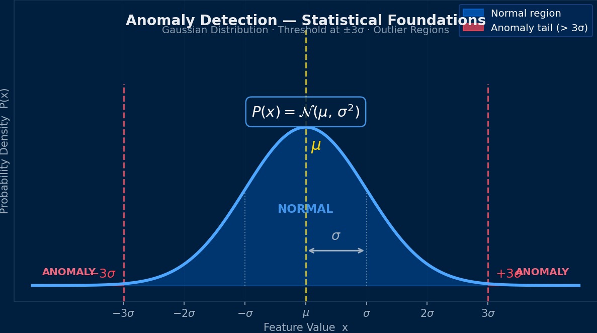
Where does anomaly detection stand statistically?
Essentially, it's the problem of "learning the probability distribution of normal data and detecting data that deviates from that distribution." From the perspective of density estimation, it involves estimating the probability density $p(\mathbf{x})$ of normal data and judging data below a threshold $\tau$ as anomalous. However, since CAE data has a high-dimensional and nonlinear structure, simple Gaussian distribution assumptions are insufficient, and nonlinear mapping via neural networks becomes necessary.
What do you do when the definition of "normal" is ambiguous?
Good question. Unsupervised anomaly detection learns only from normal data, but semi-supervised methods utilize a small number of known anomaly labels. In the context of CAE, a typical usage is to train the model using high-quality, mesh-converged simulation results as "normal" and detect results from insufficient convergence or bugs as "anomalous."
Assumptions and Applicability Limits
It's not usable for any kind of data, right?
There are several important constraints. First, there must be a sufficient amount of normal data. If the diversity of normal patterns is not covered, unknown normal patterns may be falsely detected as anomalies. Also, if the types of anomalies cannot be anticipated in advance, one must rely on unsupervised methods, but then faces the trade-off between detection sensitivity and false positive rate. Domain knowledge is essential for setting thresholds.
Are there any difficulties specific to CAE?
Yes. CAE data has vastly different scales for each physical quantity (e.g., stress at 10^8 Pa, displacement at 10^-3 m), so appropriate normalization is essential. Also, because the data representation changes with different meshes even for the same physical phenomenon, designing mesh-independent features becomes a challenge.
Theoretical Roots of Anomaly Detection—From Statistics to Manifold Learning
CAE data anomaly detection is a rather unglamorous field that originated in 1950s quality control (SPC: Statistical Process Control). The simple rule of Shewhart control charts—"outside mean ±3σ is an anomaly"—has evolved over the last 20 years into Mahalanobis distance, autoencoders, and isolation forests. Theoretically, the interesting part is the idea of "learning the manifold of the normal state." The concept of viewing points that deviate from the low-dimensional space spanned by normal data as anomalies is deeply connected to the theory of nonlinear dimensionality reduction (UMAP/t-SNE, etc.). For fluid simulations, for example, a velocity field that deviates from the manifold spanned by normal vortex behavior is identified as "anomalous," which aligns well with physical intuition.
Physical Meaning of Each Term
- Time Variation Term of Conserved Quantity: Represents the rate of change over time of the physical quantity in question. Becomes zero for steady-state problems. 【Image】When filling a bathtub with hot water, the water level rises over time—this "rate of change per time" is the time variation term. The state where the valve is closed and the water level is constant is "steady," and the time variation term is zero.
- Flux Term: Describes the spatial transport/diffusion of a physical quantity. Broadly classified into two types: convection and diffusion. 【Image】Convection is like "a river's current carrying a boat," where things are carried along by the flow. Diffusion is like "ink naturally spreading in still water," where things move due to concentration differences. The competition between these two transport mechanisms governs many physical phenomena.
- Source Term (Generation/Destruction Term): Represents the local generation or destruction of a physical quantity, i.e., external force/reaction terms. 【Image】Turning on a heater in a room "generates" thermal energy at that location. When fuel is consumed in a chemical reaction, mass is "destroyed." This term represents physical quantities injected into the system from the outside.
Assumptions and Applicability Limits
- The continuum assumption holds for the spatial scale.
- The constitutive laws of materials/fluids (stress-strain relationship, Newtonian fluid law, etc.) are within the applicable range.
- Boundary conditions are physically reasonable and mathematically well-defined.
Dimensional Analysis and Unit Systems
| Variable | SI Unit | Notes / Conversion Memo |
|---|---|---|
| Characteristic Length $L$ | m | Must match the unit system of the CAD model |
| Characteristic Time $t$ | s | For transient analysis, time step must consider CFL condition and physical time constant |
Numerical Methods and Implementation
Implementation of Main Algorithms
Specifically, what algorithms should I implement?
Let's organize the representative methods.
| Method | Principle | Strengths | Weaknesses |
|---|---|---|---|
| Autoencoder | Reconstruction Error | Strong with high-dimensional data | Threshold setting is difficult |
| Isolation Forest | Isolation via Random Splits | Fast training, scalable | Weak against local anomalies |
| One-Class SVM | Enclosing Normal Region with Hyperplane | Theoretically robust | High computational cost for large-scale data |
| LOF | Local Density Comparison | Strong against local anomalies | Affected by the curse of dimensionality |
| VAE | Deviation from Probability Distribution in Latent Space | Can quantify uncertainty | Training can be unstable |
Which one is recommended for CAE data?
For field data (stress field, temperature field, etc.), Autoencoders or VAEs are suitable. Convolutional Autoencoders, which can leverage 2D/3D spatial structures, are particularly effective. On the other hand, for anomaly detection in parameter space (deviation in the relationship between design parameters and responses), Isolation Forest or LOF are practical.
Data Preprocessing Pipeline
What should I do first when implementing?
Data preprocessing determines success or failure. The pipeline specific to CAE data is as follows.
1. Scaling: Normalize each physical quantity individually using Min-Max or Z-score normalization. Essential if mixing stress and displacement.
2. Feature Extraction: There are methods to extract scalar features (maximum, mean, standard deviation, gradient magnitude) from field data, and methods to treat field data directly as images.
3. Missing Value Handling: Removal or flagging of NaN/Inf from diverged calculation cases.
4. Dimensionality Reduction: Another approach is to reduce dimensions using PCA or t-SNE before anomaly detection.
Why use HDF5?
For efficiently reading and writing large-scale CAE data (tens of thousands of cases, millions of nodes per case) as NumPy arrays, HDF5's chunked I/O and compression features are indispensable. It's not uncommon to be over 10 times faster compared to CSV reading.
Implementation Tips
Please tell me specific tips for writing in Python.
- scikit-learn's IsolationForest and LocalOutlierFactor can be used as-is.
- When building an autoencoder with PyTorch, the dimension of the bottleneck layer is important. Start with about 1/10 to 1/20 of the input dimension.
- Batch size: too small leads to unstable training, too large causes anomaly features to be averaged out and buried. Around 32 to 128 is a good guideline.
- For the anomaly score threshold, the 95th or 99th percentile of the reconstruction error on training data is often used.
Validation Methods
How do you evaluate the performance of anomaly detection?
The basic metrics are Precision, Recall, F1 Score, and AUC-ROC. However, in the CAE context, anomalous data is often extremely scarce, so the PR curve (Precision-Recall curve) is often more appropriate than the ROC curve. Also, domain expert confirmation of whether detected anomalies are physically meaningful is essential.
Anomalies Autoencoders "Overlook"—The Pitfall of Reconstruction Error
The basic idea of anomaly detection using autoencoders is "a model trained on normal data cannot reconstruct anomalies → large reconstruction error = anomaly." However, in practice, there are unexpected pitfalls. For example, in a certain automaker's crash simulation quality check, the autoencoder falsely identified "rare but normal" complex deformation patterns as anomalies. The model hadn't fully learned the diversity of normality. As countermeasures, methods like β-VAE (Variational Autoencoder) to regularize the latent space, or directly learning a hypersphere of normal data like Deep SVDD (Support Vector Data Description), are said to be effective.
Low-Order Elements
Low computational cost and easy to implement, but accuracy is limited. May produce large errors with coarse meshes.
Higher-Order Elements
Achieves higher accuracy with the same mesh. Computational cost increases, but the required number of elements is often reduced.
Newton-Raphson Method
Standard method for nonlinear problems. Quadratic convergence within the convergence radius. Convergence judged by $||R|| < \epsilon$.
Time Integration
Explicit Method: Conditionally stable (CFL Condition). Implicit Method: Unconditionally stable but requires solving simultaneous equations at each step.
Image of Discretization
Numerical methods are similar to "taking a photo with a digital camera." It represents the continuous real-world scenery (continuum) with a finite number of pixels (elements/cells). Increasing the number of pixels (mesh density) improves image quality (accuracy), but also increases file size (computational cost). Finding the optimal balance is where practical skill comes in.
Practical Guide
Overall Analysis Flow
When implementing CAE data anomaly detection in practice, where should I start?
The overall flow is as follows.
1. Clarify the Objective: Decide what to define as an anomaly. The method changes depending on whether it's detecting numerical errors from the solver or detecting deviations in design parameters.
2. Build a Normal Database: Collect reliable simulation results that have been verified for mesh convergence and validated (V&V).
3. Feature Design: Choose between scalar features or field data according to the target.
4. Model Training and Threshold Determination: Confirm generalization performance through cross-validation while balancing false positive rate and miss rate.
5. Operation and Continuous Improvement: Regularly update the model with new data.
Building the normal database seems like the hardest part.
Exactly. The quality of the normal data determines the overall reliability of the model. In practice, analysis results verified by experienced CAE engineers as "guaranteed" are used as normal labels. The golden rule is to only adopt results that have undergone mesh convergence verification, force balance verification, and comparison with theoretical solutions.
Best Practices
Please tell me tips to avoid failure.
- Clearly define the scope of application for the anomaly detection model. Do not apply it to analysis types (linear static analysis, heat conduction, etc.) different from those used in training.
- Consider making thresholds adaptive based on location in parameter space, not fixed values. The range of "normal" differs between stress concentration areas and uniform stress areas.
- Always implement a workflow where detected anomalies are confirmed by a human. Full automation is still too risky.
- Log anomaly detection results, analyze false positive patterns, and continuously improve the model.
Use Cases
In what actual situations is it being used?
Representative use cases are as follows.
| Use Case | Detection Target |
|---|