ML Uncertainty Quantification
ML Uncertainty Quantification: Theoretical Foundations
Overview
What does it mean when machine learning predictions have "uncertainty"?
When using ML surrogate models in CAE, it's important to output not just the predicted value but also "how reliable that prediction is" simultaneously. Uncertainty Quantification (UQ) is a technique that attaches confidence intervals to predictions, ensuring the reliability of decision-making.
Why is it particularly important in CAE?
Because setting safety factors and determining compliance with standards require not just predicted values but also error margins. It's insufficient for an ML model to simply say "the maximum stress of this part is 200 MPa"; it must be able to say "200 MPa ± 15 MPa (95% confidence interval)" to be usable for design decisions.
Classification of Uncertainty
Are there different types of uncertainty?
They can be broadly divided into two types.
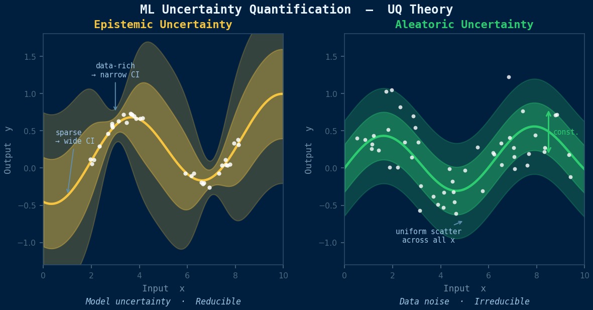
- Aleatoric Uncertainty (Stochastic Uncertainty): Noise inherent in the data itself. Caused by measurement errors and manufacturing variations. Cannot be reduced even by increasing data.
- Epistemic Uncertainty (Epistemological Uncertainty): Uncertainty arising from the model's lack of knowledge. Becomes larger in regions with little training data. Can be reduced by increasing data.
How are they separated mathematically?
They are separated using methods like MC Dropout or Deep Ensemble. Let $\hat{y}_t$ be the prediction from the $t$-th forward pass out of $T$ passes, and $\hat{\sigma}_t^2$ be the predictive variance for each pass, then:
The first term is the variance due to uncertainty in model parameters, and the second term is the variance due to data noise.
Bayesian Inference Framework
Please explain the relationship with the Bayesian approach.
In strict Bayesian inference, we find the posterior distribution $p(\theta|\mathcal{D})$ of parameters $\theta$ and compute the predictive distribution via integration.
However, this integral is analytically intractable, so we use MC Dropout (interpreting dropout as a Bayesian approximation) or Deep Ensemble (approximating with predictive distributions of multiple models). Gaussian Process Regression naturally fits into this framework, but scalability becomes an issue with large-scale data.
Bayesian Statistics and ML Uncertainty—The Philosophy of "Prediction as Probability"
"How reliable is this simulation result?"—The theory of ML Uncertainty Quantification (UQ) directly confronts this question. Traditional neural networks only return point estimates (a single answer) and do not provide confidence intervals. Bayesian Neural Networks (BNNs) treat the model parameters themselves as probability distributions and output "a distribution of answers." Theoretically elegant, but computing the true posterior distribution for NNs with millions of parameters is impossible (NP-hard), so approximations via variational inference (ELBO maximization) or MCMC are used. In CAE applications, outputs like "within ±15MPa at 95% confidence interval" for stress peak predictions in crash simulations are demanded in insurance/certification contexts, and pressure from regulatory bodies is accelerating UQ research.
Computational Methods for ML Uncertainty Quantification
Implementation of Major Methods
How is it actually implemented?
Let's summarize the representative methods.
| Method | Principle | Ease of Implementation | Computational Cost |
|---|---|---|---|
| MC Dropout | Keep dropout active during inference and predict T times | Easy | T times |
| Deep Ensemble | Train M independent models | Moderate | M times |
| Bayesian NN (VI) | Approximate parameter posterior distribution via Variational Inference | Difficult | 2~3 times |
| Gaussian Process Regression | Non-parametric regression via kernel methods | Moderate | $O(N^3)$ |
| Evidential DL | Simultaneously estimate aleatoric/epistemic uncertainty using Dirichlet distribution | Moderate | 1 times |
MC Dropout seems the easiest.
Exactly. If you already have an NN with dropout, you just need to predict T times (50~100 times) during inference while keeping the model in model.train() mode. The average becomes the prediction, and the variance becomes the uncertainty. However, note that the dropout rate setting affects calibration.
Calibration
How do you confirm if the uncertainty estimation is "correct"?
Calibration is a key concept. If 95% of the actual data falls within the 95% confidence interval, the model is said to be "well-calibrated."
- Calibration Curve: Plots expected confidence level vs. actual coverage rate.
- Expected Calibration Error (ECE): A quantitative metric for calibration.
- Temperature Scaling: A post-processing technique to improve calibration.
What happens if calibration is off?
Overconfidence (confidence intervals too narrow) is dangerous. For example, if a "95% confidence interval" actually only covers 70% of the data, it can lead to erroneous design decisions. Temperature scaling is a simple post-processing technique that just divides the logits of the output layer by a temperature parameter $T$, but it is very effective for improving calibration.
Output Format Design
What output format is easy for CAE engineers to use?
- Output stress prediction values and standard deviations for each node in VTK format, and visualize them as an uncertainty map in ParaView.
- Use the 95th percentile value of the predictive distribution as a "worst-case estimate" for design decisions.
- Highlight regions where uncertainty exceeds a threshold to automatically identify areas requiring additional full FEM analysis.
Turning Dropout On During Inference—The Trick of MC Dropout
The easiest method to implement as an approximation to Bayesian Neural Networks is "MC Dropout." This technique, published by Gal & Ghahramani at NIPS in 2016, involves not turning dropout off during inference for an existing NN with dropout (it's usually off during inference), and instead executing T stochastic forward passes and using their variance as a proxy for uncertainty. Its overwhelming strength is that implementation requires only a few lines of code changes. However, there are pitfalls: if the dropout rate is too low, uncertainty is underestimated; if it's too high, accuracy drops. When applying it to CAE surrogate models, you must always perform a verification test to ensure that uncertainty correctly becomes larger at the edges of the input space where training data is scarce (extrapolation regions). Neglecting this can create models that "seem trustworthy but are not."
ML Uncertainty Quantification in Practice
Workflow for Practical Use
Please tell me the steps to use an ML model with UQ in practice.
1. Understand the uncertainty in the training data: First, quantify the uncertainty in the input data (material constants, loads, etc.) and the mesh error in the output data (FEM solutions).
2. Select an ML model compatible with UQ: Deep Ensemble (relatively easy to implement and stable performance) is the first candidate.
3. Verify calibration: Confirm the coverage rate of the confidence interval on test data.
4. Set design decision criteria: Decide in advance how to set safety factors that incorporate uncertainty.
5. Continue monitoring: Periodically check if calibration is maintained during operation.
Best Practices
What are the key points to avoid failure?
- Utilize the fact that epistemic uncertainty becomes larger in regions with little training data as a "feature." It can automatically detect the extrapolation limits of the surrogate model.
- Consider uncertainty propagation. Track the chain: input parameter uncertainty → ML model uncertainty → design metric uncertainty.
- "High uncertainty" means "unknown," not "wrong." It's important to share this distinction within the team.
- Always evaluate calibration on an independent test set. Evaluating on training data is meaningless.
Use Cases
What specific effects does it have?
| Scenario | Without UQ | With UQ |
|---|---|---|
| Surrogate Optimization | Optimal solution converges to non-physical regions | Obtains reliable optimal solutions by avoiding regions with high uncertainty |
| Digital Twin | Reliability of predictions is unknown | Alerts when prediction accuracy degrades in specific locations |
| Safety Assessment | Safety factor judged based on point estimate | Safety factor judged based on upper probability of predictive distribution |
| Active Learning | Next sample point chosen arbitrarily | Efficiently collects data by selecting the point with maximum uncertainty |
Fusion Reactor Design and UQ—The Challenge of Quantifying "Uncomputable Unknowns"
Fusion reactor design is full of uncertainties. Plasma behavior is nonlinear and chaotic, and there is extremely little measured data on material properties under high neutron irradiation environments. In the EUROFUSION project, Gaussian Process regression-based UQ is applied to the thermal load analysis of ITER's first wall (the wall in contact with plasma). By setting uncertainty distributions for physical parameters and evaluating thousands of Monte Carlo samples with a GP surrogate, the probability distribution of the risk of wall melting is estimated. A practical point is that "the setting of parameter uncertainty" greatly influences the results—design decisions change depending on whether ±10% or ±30% uncertainty is assumed for the material's thermal conductivity. The real skill lies in how to incorporate experts' subjective judgments into Bayesian prior distributions.
ML Uncertainty Quantification: Software & Solver Comparison
| Tool | Type | UQ Method | Features |
|---|---|---|---|
| GPyTorch | OSS | Gaussian Process | PyTorch-based, GPU support, scalable |
| Uncertainty Toolbox | OSS | Evaluation Metrics | Standard tool for calibration evaluation |
| TensorFlow Probability | OSS | Bayesian NN, VI | TF integrated, probabilistic programming |
| Pyro/NumPyro | OSS | Probabilistic Programming | Flexible Bayesian modeling |
| UQLab | Academic | PCE, kriging |