ML Adaptive Mesh Refinement
ML Adaptive Mesh Refinement: Theoretical Foundations
Overview
Teacher! Today's topic is about ML adaptive mesh refinement, right? What is it?
It's a method that uses ML to predict which regions should be refined based on error estimates or solution gradient patterns. It reduces the computational cost of a posteriori error estimation while enabling efficient h-refinement.
Ah, I see! So that's how error estimates and solution gradients work.
Governing Equations
Expressing this mathematically, it looks like this.
Hmm, just the equation alone doesn't really click... What does it represent?
ML prediction model:
Theoretical Foundation
I've heard of "theoretical foundation," but I might not fully understand it...
ML adaptive mesh refinement is an important technique aiming to fuse data-driven approaches with physics-based modeling. While computational cost is a major bottleneck in traditional CAE analysis, introducing ML adaptive mesh refinement can significantly improve the trade-off between computational efficiency and prediction accuracy. The mathematical foundation of this method is based on function approximation theory and statistical learning theory, with generalization performance guarantees and rigorous analysis of convergence being key theoretical research topics. Particularly, dealing with the "curse of dimensionality" in high-dimensional input spaces is crucial for practical application, and approaches like dimensionality reduction and leveraging sparsity are important.
Now I understand what my senior meant when they said, "At least make sure you do adaptive mesh refinement properly."
Details of Mathematical Formulation
Next is "Details of Mathematical Formulation"! What is this about?
It presents the basic mathematical framework for applying machine learning models to CAE.
Loss Function Composition
What does "loss function composition" specifically mean?
In AI×CAE, the loss function is composed as a weighted sum of a data-driven term and a physics constraint term:
Here, $\mathcal{L}_{\text{data}}$ is the squared error with observed data, $\mathcal{L}_{\text{physics}}$ is the residual of the governing equation, and $\mathcal{L}_{\text{reg}}$ is a regularization term. Adjusting the weight parameters $\lambda$ greatly affects learning stability and accuracy.
Generalization Performance and Extrapolation Problem
Please tell me about "Generalization Performance and the Extrapolation Problem"!
The biggest challenge for surrogate models is prediction accuracy outside the range of training data (extrapolation region). Incorporating physical laws can improve extrapolation performance, but complete guarantees are difficult.
Curse of Dimensionality
Please tell me about the "Curse of Dimensionality"!
When the dimension of the input parameter space is high, the required number of samples increases exponentially. Efficient sample placement through Active Learning or Latin Hypercube Sampling (LHS) is extremely important.
Assumptions and Applicability Limits
Isn't this formula universal? When can't it be used?
- The training data must sufficiently represent the physics of the analysis target.
- The relationship between input parameters and output must be smooth (if discontinuities exist, domain partitioning is necessary).
- Reducing computational cost is the main objective; conventional solvers should be used in conjunction for final verification requiring high accuracy.
- If the quality of training data (mesh-converged, V&V completed) is insufficient, model reliability decreases.
Ah, I see! So that's how the training data and analysis target work.
Dimensionless Parameters and Dominant Scales
Teacher, please tell me about "Dimensionless Parameters and Dominant Scales"!
Understanding the dimensionless parameters governing the physical phenomenon being analyzed forms the basis for appropriate model selection and parameter setting.
- Péclet Number Pe: Relative importance of convection vs. diffusion. Pe >> 1 indicates convection dominance (stabilization techniques required).
- Reynolds Number Re: Ratio of inertial forces to viscous forces. A fundamental parameter for fluid problems.
- Biot Number Bi: Ratio of internal conduction to surface convection. For Bi < 0.1, the lumped capacitance method is applicable.
- Courant Number CFL: Indicator of numerical stability. For explicit methods, CFL ≤ 1 is required.
Ah, I see! So that's how the physics of the analysis target works.
Verification via Dimensional Analysis
Please tell me about "Verification via Dimensional Analysis"!
For order-of-magnitude estimation of analysis results, dimensional analysis based on Buckingham's Π theorem is effective. Using characteristic length $L$, characteristic velocity $U$, and characteristic time $T = L/U$, the order of each physical quantity is estimated beforehand to confirm the validity of the analysis results.
I see. So if we can do that for the physics of the analysis target, we're basically okay to start?
Classification of Boundary Conditions and Mathematical Characteristics
I've heard that if you get the boundary conditions wrong, everything fails...
| Type | Mathematical Expression | Physical Meaning | Example |
|---|---|---|---|
| Dirichlet Condition | $u = u_0$ on $\Gamma_D$ | Specification of variable value | Fixed wall, specified temperature |
| Neumann Condition | $\partial u/\partial n = g$ on $\Gamma_N$ | Specification of gradient (flux) | Heat flux, force |
| Robin Condition | $\alpha u + \beta \partial u/\partial n = h$ | Linear combination of variable and gradient | Convective heat transfer |
| Periodic Boundary Condition | $u(x) = u(x+L)$ | Spatial periodicity | Unit cell analysis |
Choosing appropriate boundary conditions is directly linked to solution uniqueness and physical validity. Insufficient boundary conditions lead to an ill-posed problem, while excessive ones cause contradictions.
Yeah, you're doing great! Actually trying things out is the best way to learn. If you don't understand something, feel free to ask anytime.
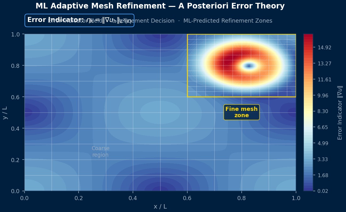
Theory of Adaptive Mesh Refinement—When to Use A Posteriori Error Estimators vs. ML
The theoretical foundation of Adaptive Mesh Refinement (AMR) is the "a posteriori error estimator" in finite element analysis. The Zienkiewicz-Zhu (ZZ) estimator is a prime example; it calculates the stress discontinuity between adjacent elements after analysis and uses the magnitude of discontinuity (i.e., where the solution is coarse) as an indicator for refinement. While this method theoretically guarantees an error upper bound, its drawback is the double computational cost because refinement occurs after running the analysis. This is where ML comes in: it is used as an "a priori estimator" that predicts "this region will likely need refinement" based solely on CAD geometry before analysis, generating an appropriate mesh from the start to achieve convergence in a single analysis. A hybrid strategy combining a priori and a posteriori approaches is the most powerful in practice.
Computational Methods for ML Adaptive Mesh Refinement
Details of Numerical Methods
Specifically, what algorithm is used to solve ML adaptive mesh refinement?
Explains the numerical methods and algorithms for implementing ML adaptive mesh refinement.
I see... Adaptive mesh refinement seems simple at first glance, but it's actually very profound.
Discretization and Calculation Procedure
How do you actually solve this equation on a computer?
As data preprocessing, normalization/standardization of input features is crucial. Since CAE data scales vary greatly for different physical quantities, appropriate selection of Min-Max normalization or Z-score normalization is necessary. For learning algorithm selection, the appropriate method should be chosen based on data volume, dimensionality, and degree of nonlinearity.
Implementation Considerations
What is the most important thing to be careful about when using ML adaptive mesh refinement in practice?
Implementation using the Python ecosystem (scikit-learn, PyTorch, TensorFlow) is common. Keys to implementation are learning acceleration via GPU parallelization, automatic hyperparameter tuning, and preventing overfitting through cross-validation. Using the HDF5 format is recommended for efficient I/O processing of large-scale CAE data.
Verification Methods
Teacher, please tell me about "Verification Methods"!
It's important to use k-fold cross-validation, Leave-One-Out method, and holdout method appropriately for the purpose, and to evaluate prediction performance comprehensively using coefficient of determination R², RMSE, MAE, and maximum error.
Now I understand what my senior meant when they said, "At least make sure you do cross-validation properly."
Code Quality and Reproducibility
What is the most important thing to be careful about when using ML adaptive mesh refinement in practice?
Ensure code quality and experiment reproducibility by introducing version control (Git), automated testing (pytest), and CI/CD pipelines. Strictly enforce dependency version pinning (requirements.txt) to make rebuilding the computational environment easy. Ensuring result reproducibility by fixing random seeds is also an important implementation practice.
Ah, I see! So that's how version control works.