Adaptive Mesh Refinement (AMR)
Theory: refine only where needed
Overview
I want to simulate a droplet hitting a water surface, but resolving the interface finely needs tens of millions of cells.
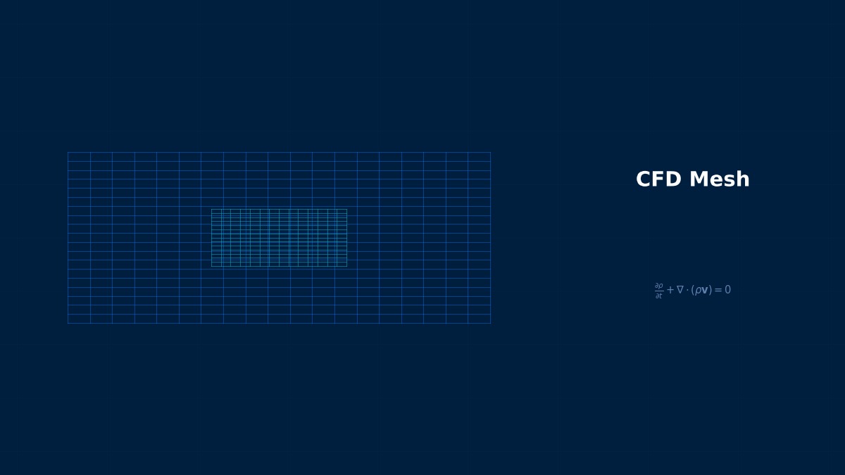
Because you're using the same fineness everywhere, though the interface is a tiny part of the domain. AMR watches the solution during the run, splitting cells only where values change sharply — interfaces, shocks — and leaving quiet regions coarse. When the interface moves, the fine region moves with it. Used well, it often cuts cell counts by more than an order of magnitude at the same accuracy. But the choice of refinement indicator and the handling of fine–coarse boundaries need care.
Refinement indicator
$h_i$ is cell size and the second derivative the solution's curvature. Linear interpolation error scales roughly with $h^2$ times curvature, so cells where this is large are split and cells where it is small are coarsened. Real solvers use problem-appropriate indicators — gradient magnitude, volume fraction (interfaces), vorticity and so on.
Effect on time step
In explicit schemes the time step is set by the smallest cell. Each AMR level halves cell size and time step. Local time stepping (subcycling), advancing only fine cells with small steps, keeps total run time down.
Born of astrophysics and shock waves
AMR took shape in the 1980s when Berger and Oliger proposed layering blocks of finer grids for hyperbolic equations (those governing waves such as shocks), extended by Berger and Colella to shock-wave computations. It proved especially valuable in astrophysics — stellar explosions, galaxy formation — where small regions change violently within vast domains. Today it is a standard feature of commercial CFD for free-surface flow, combustion, jets and more.
Worked example: cells needed to resolve a sharp front
On [0, 1], the sharp front $u = \tanh((x-0.5)/w)$ is represented by linear interpolation within cells. The number of cells needed to bring maximum error below a threshold is compared for a uniform grid and for an approach that bisects only cells with large error (AMR).
| Front width | Error tolerance | Uniform | AMR | Ratio | Finest cell |
|---|---|---|---|---|---|
| 0.01 | 1% | 317 | 26 | 12 | 0.0020 |
| 0.01 | 0.1% | 992 | 56 | 18 | 0.0010 |
| 0.002 | 1% | 1,545 | 30 | 52 | 0.00049 |
| 0.002 | 0.1% | 5,009 | 70 | 72 | 0.00012 |
The sharper the front, the bigger AMR's advantage.
Right. A uniform grid must be fine everywhere to match the front width, while AMR refines only near the front. This is 1D; in 2D and 3D uniform counts grow with the square or cube of fineness while AMR only refines near the front line or surface, so the gap widens further. AMR cells vary in size, though, so per-cell cost and data management are heavier than on uniform grids — the cell-count ratio isn't directly the run-time ratio.
Use and pitfalls
Setup points
- Pick an indicator that best captures the phenomenon (volume fraction for interfaces, pressure gradient for shocks, vorticity for vortices).
- Set the maximum refinement level and check the finest cell can resolve the smallest feature.
- Set refinement frequency; fronts moving more than a cell between adaptations escape the fine region.
- Vary thresholds and confirm results don't change (mesh independence with AMR).
Pitfalls
- Level interfaces: keep neighbouring size ratios at 2:1 or less, with corrections so conserved quantities don't leak.
- Near walls: inflation layers and AMR can conflict; near-wall regions often keep a fixed mesh.
- Parallel load: fine regions clustering on some processors unbalance the load; rebalancing is needed.
“The refinement lags behind the front”
Tracking fast flames or shocks with AMR, the fine region can fail to keep up and the front escapes into coarse cells. It then smears, the indicator weakens and refinement stops — a vicious circle. Shorten the adaptation interval or refine a margin ahead of the front (a buffer layer). AMR settings that work for stationary features may fail for moving ones, so check front and fine-region positions over time.
Common mistakes
Mistakes and fixes
| Mistake | Effect | Fix |
|---|---|---|
| Indicator mismatched to phenomenon | Needed regions stay coarse | Choose a representative quantity |
| Adaptation interval too long | Front escapes to coarse cells | Shorter interval, buffer layer |
| Ignoring threshold sensitivity | Setting-dependent results | Vary thresholds and compare |
| Estimating time from cell ratio | Run time underestimated | Account for small steps and overhead |
| Ignoring conservation at level interfaces | Mass and other quantities leak | Use conservative corrections |
I'd like to explore mesh resolution myself.
Try the mesh convergence tool and mesh independence study tool for resolution versus error and the CFD mesh quality checker for grid quality. Other meshing techniques are covered in overset (Chimera) grids, inflation layers and polyhedral meshes, and verification in mesh independence.
Related Topics
Experience the theory firsthand with the interactive simulator for this field
All Simulators