CAE Control via Reinforcement Learning
Overview
Professor! Today let us talk about CAE control using reinforcement learning, right? What is it about?
CAE Control via Reinforcement Learning: Theoretical Foundations
A method that uses Reinforcement Learning (RL) for optimal control of simulation parameters and active flow control. The environment is defined as a CFD simulation, and the policy is optimized based on reward signals.
Wait, wait, so you're saying Reinforcement Learning can be used in cases like this too?
Governing Equations
Expressing this mathematically, it looks like this.
Hmm, just the equation alone doesn't really click for me... What does it represent?
Policy Gradient Method:
Theoretical Foundation
I've heard of "Theoretical Foundation," but I might not fully understand it...
CAE control using Reinforcement Learning is an important method aiming for the fusion of data-driven approaches and physics-based modeling. While computational cost is a major bottleneck in conventional CAE analysis, introducing CAE control via Reinforcement Learning can significantly improve the trade-off between computational efficiency and prediction accuracy. The mathematical foundation of this method is based on function approximation theory and statistical learning theory, with theoretical research topics including guarantees of generalization performance and rigorous analysis of convergence. Particularly, dealing with the "curse of dimensionality" in high-dimensional input cases is a key practical challenge, and approaches like dimensionality reduction and leveraging sparsity are important.
Your explanation is easy to understand! The haze around Reinforcement Learning has cleared up.
Details of Mathematical Formulation
Next is "Details of Mathematical Formulation"! What kind of content is this?
It shows the basic mathematical framework for applying machine learning models to CAE.
Loss Function Composition
What does "Loss Function Composition" mean specifically?
The loss function in AI×CAE is composed as a weighted sum of a data-driven term and a physics constraint term:
Here, $\mathcal{L}_{\text{data}}$ is the squared error with observed data, $\mathcal{L}_{\text{physics}}$ is the residual of the governing equations, and $\mathcal{L}_{\text{reg}}$ is the regularization term. Adjusting the weight parameters $\lambda$ greatly affects learning stability and accuracy.
Generalization Performance and Extrapolation Problem
Please tell me about "Generalization Performance and the Extrapolation Problem"!
The biggest challenge for surrogate models is prediction accuracy outside the range of training data (extrapolation region). Incorporating physical laws can improve extrapolation performance, but complete guarantees are difficult.
Curse of Dimensionality
Please tell me about the "Curse of Dimensionality"!
When the dimensionality of the input parameter space is high, the required number of samples increases exponentially. Efficient sample placement using Active Learning or Latin Hypercube Sampling (LHS) is extremely important.
Assumptions and Applicability Limits
Isn't this formula universal? When can't it be used?
- The training data must sufficiently represent the physics of the analysis target.
- The relationship between input parameters and output must be smooth (if discontinuities exist, domain partitioning is necessary).
- Reducing computational cost is the main objective; conventional solvers should be used in conjunction for final verification requiring high accuracy.
- If the quality of training data (mesh-converged, V&V completed) is insufficient, model reliability decreases.
Ah, I see! So that's how the mechanism of training data representing the analysis target works.
Dimensionless Parameters and Dominant Scales
Professor, please tell me about "Dimensionless Parameters and Dominant Scales"!
Understanding the dimensionless parameters governing the physical phenomenon being analyzed forms the basis for appropriate model selection and parameter setting.
- Péclet Number Pe: Relative importance of convection vs. diffusion. Pe >> 1 indicates convection-dominated (stabilization techniques required).
- Reynolds Number Re: Ratio of inertial forces to viscous forces. A fundamental parameter for fluid problems.
- Biot Number Bi: Ratio of internal conduction to surface convection. For Bi < 0.1, the lumped capacitance method is applicable.
- Courant Number CFL: Indicator of numerical stability. For explicit methods, CFL ≤ 1 is required.
Ah, I see! So that's how the mechanism of the analysis target's physical phenomenon works.
Verification via Dimensional Analysis
Please tell me about "Verification via Dimensional Analysis"!
For order-of-magnitude estimation of analysis results, dimensional analysis based on Buckingham's Π theorem is effective. Using characteristic length $L$, characteristic velocity $U$, and characteristic time $T = L/U$, the order of each physical quantity is estimated in advance to confirm the validity of the analysis results.
I see. So if the analysis target's physical phenomenon is understood, then it's basically okay to start?
Classification of Boundary Conditions and Mathematical Characteristics
I've heard that if you get the boundary conditions wrong, everything falls apart...
| Type | Mathematical Expression | Physical Meaning | Example |
|---|---|---|---|
| Dirichlet Condition | $u = u_0$ on $\Gamma_D$ | Specification of variable value | Fixed wall, specified temperature |
| Neumann Condition | $\partial u/\partial n = g$ on $\Gamma_N$ | Specification of gradient (flux) | Heat flux, force |
| Robin Condition | $\alpha u + \beta \partial u/\partial n = h$ | Linear combination of variable and gradient | Convective heat transfer |
| Periodic Boundary Condition | $u(x) = u(x+L)$ | Spatial periodicity | Unit cell analysis |
Choosing appropriate boundary conditions is directly linked to solution uniqueness and physical validity. Insufficient boundary conditions lead to an ill-posed problem, while excessive ones create contradictions.
I've grasped the overall picture of CAE control using Reinforcement Learning! I'll try to be mindful of it in my practical work starting tomorrow.
Yeah, you're on the right track! Actually getting your hands dirty is the best way to learn. If you have any questions, feel free to ask anytime.
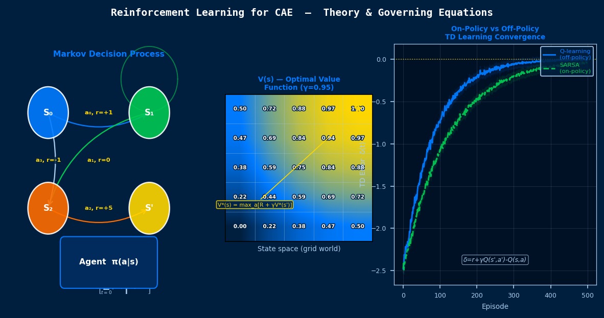
Markov Decision Processes and CAE—Defining "Continuous Design Improvement" Mathematically
The mathematical foundation of Reinforcement Learning (RL) is the Markov Decision Process (MDP). It defines decision-making problems as a quadruple of State, Action, Reward, and Transition probability. In applications to CAE design optimization, the state becomes simulation results (stress, displacement, temperature distribution, etc.), the action becomes the change amount of design parameters, and the reward becomes the improvement amount of performance indicators. Theoretically interesting is the "delayed reward" structure unique to CAE problems: when it takes several hours from taking an action (parameter change) until the simulation completes, no reward is obtained during that time. To address this, methods combining model-based RL (fast approximation of simulation using a world model) with surrogate models are being researched, making it one of the most active fields bridging theory and implementation. Particularly, dealing with the "curse of dimensionality" in high input dimensions is a key practical challenge, and approaches like dimensionality reduction and leveraging sparsity are important.
Computational Methods for CAE Control via Reinforcement Learning
Explains numerical methods and algorithms for implementing CAE control using Reinforcement Learning.
Ah, I see! So that's how the mechanism of Reinforcement Learning works.
Discretization and Calculation Procedure
How do you actually solve this equation on a computer?
As data preprocessing, normalization/standardization of input features is important. Since CAE data scales vary greatly by physical quantity, appropriate selection of Min-Max normalization or Z-score normalization is necessary. In selecting learning algorithms, appropriate methods should be chosen according to data volume, dimensionality, and degree of nonlinearity.
Implementation Considerations
What is the most important thing to be careful about when using CAE control via Reinforcement Learning in practical work?
Implementation using the Python ecosystem (scikit-learn, PyTorch, TensorFlow) is common. Keys to implementation are learning acceleration via GPU parallelization, automatic hyperparameter tuning, and preventing overfitting via cross-validation. Utilizing the HDF5 format is recommended for efficient I/O processing of large-scale CAE data.
Verification Methods
Professor, please tell me about "Verification Methods"!
It's important to use k-fold cross-validation, Leave-One-Out method, and holdout method appropriately for the purpose, and to evaluate prediction performance comprehensively using coefficient of determination R², RMSE, MAE, and maximum error.
I understand now why my senior said, "At least do cross-validation properly."
Code Quality and Reproducibility
What is the most important thing to be careful about when using CAE control via Reinforcement Learning in practical work?
Ensure code quality and experiment reproducibility by introducing version control (Git), automated testing (pytest), and CI/CD pipelines. Strictly enforce dependency library version pinning (requirements.txt) to make rebuilding the computational environment easy. Ensuring result reproducibility by fixing random seeds is also an important implementation practice.
Ah, I see! So that's how version control works.
Implementation Algorithm Details
I want to know a bit more about what's happening behind the scenes of the calculation!