Arc Welding Simulation
Theoretical Foundations of Arc Welding Simulation
What the Analysis Predicts — Three Tiers
Arc welding simulation divides into three tiers according to purpose. (1) Thermal analysis: predicting the temperature history produced by a moving heat source (weld pool shape, HAZ width, cooling rate). (2) Thermo-elastoplastic analysis: taking that temperature history as input to predict welding distortion and residual stress. (3) Microstructure and property prediction: estimating phase transformation, hardness and cracking susceptibility from the cooling rate. The main battleground in industry is (2), prediction of distortion and residual stress, because it maps directly onto manufacturing problems: "the parts no longer fit together after welding", "residual stress eats into fatigue life". One-way coupling from thermal to mechanical (the effect of deformation on the thermal field neglected) is generally held to be sufficient.
The Moving Heat Source Model — Goldak's Double Ellipsoid
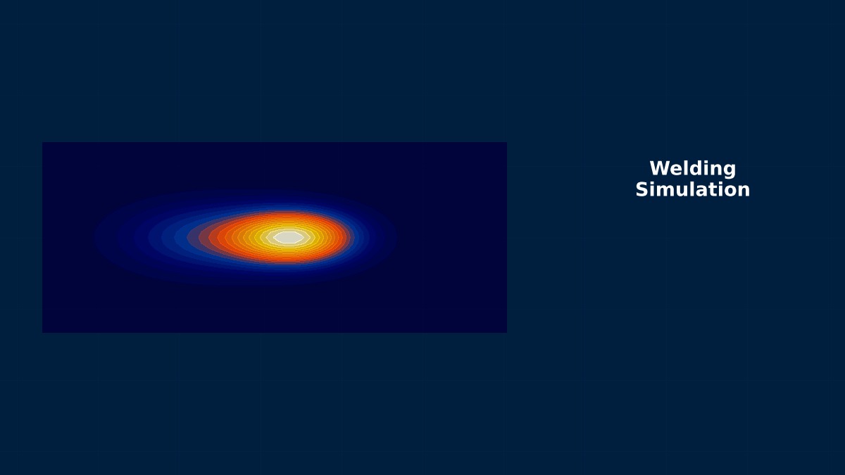
The heat input of the arc is not solved from first principles; the standard is to impose a calibratable equivalent heat source model. The de facto industry standard is Goldak's double-ellipsoid source, which moves a volumetric heat source made of ellipsoid halves of different length ahead of and behind the travel direction.
$$ q_f(x,y,z) = \frac{6\sqrt{3}\, f_f\, \eta Q}{a_f b c\, \pi\sqrt{\pi}} \exp\!\left( -\frac{3x^2}{a_f^2} - \frac{3y^2}{b^2} - \frac{3z^2}{c^2} \right) $$
\( Q = UI \) is the arc power, \( \eta \) the thermal efficiency (process dependent: roughly 0.6–0.8 for TIG, 0.75–0.9 for MAG), and \( a_f, a_r, b, c \) the semi-axes of the ellipsoids. These parameters are not physical constants but calibration targets — they acquire predictive power only once they have been fitted to macrographs of the weld pool cross section and to thermocouple measurements. Taking published values as they stand is the single largest source of failure in welding simulation.
Phase Transformation in Steel, a Physics of Its Own
In carbon and low-alloy steels, martensitic and bainitic transformation during cooling brings volumetric expansion and transformation plasticity, which qualitatively changes the residual stress distribution (transformation expansion relaxes or even reverses the tensile residual stress). It is unnecessary for austenitic stainless steels and aluminium, but a residual stress prediction that ignores phase transformation in a hardenable steel can get even the sign wrong. That the essential physics changes with the material system is the core of what separates welding simulation from ordinary thermal stress analysis.
Numerical Methods
The Detailed Approach — Transient Thermo-Elastoplastic Analysis
A detailed analysis of one to a few passes proceeds as a transient thermal analysis with a moving heat source, followed by an elastoplastic analysis loaded by the resulting temperature history. The numerical essentials are as follows.
- Mesh — resolve the weld pool with several elements near the bead (of the order of 1–2 mm) and coarsen away from it. Deposited metal is added pass by pass through element birth and death (quiet elements)
- Time step — while the heat source is passing, keep it below the heat source dimension divided by the travel speed. Expand it logarithmically during the cooling period
- High-temperature material data — temperature-dependent properties up to near the melting point (yield stress, Young's modulus, thermal properties) are mandatory. State explicitly how the high-temperature range is extrapolated where the data run out (clipping the yield stress at a floor value, for instance)
- Strain hardening and annealing — without the annealing function that resets the hardening history on reheating (annealing temperature), stress is overestimated in multi-pass welds
Approximation for Large Structures — the Inherent Strain Method
A moving heat source analysis of every pass is impossible for a ship hull or a construction-machine frame tens of metres long. The practical standard is the inherent strain method: the shrinkage and angular distortion per unit length of weld line (the inherent strain) obtained from a detailed analysis, or from measurement, is applied as an initial strain to an elastic analysis of the whole structure, giving the overall distortion in a single solve. Where the transient approach "solves one joint with minute-scale physics", the inherent strain method "solves the overall distortion of a thousand weld lines in minutes" — an asset-type technique in which the organisation with the better joint library (inherent strain tabulated by joint type × plate thickness × heat input) is the stronger one.
Practical Procedure for Heat Source Calibration
- Run a bead-on-plate test at production conditions (current, voltage, travel speed) and collect cross-sectional macrographs plus a few thermocouple readings (outer edge of the HAZ)
- Identify the efficiency η and the ellipsoid parameters so that the weld pool cross section (width and penetration depth) matches
- Cross-validate against the thermocouple temperature histories (peak and cooling rate) — if the cross section matches but the history does not, redo the parameter identification
- Use the calibrated heat source within the range of conditions it was calibrated for (roughly ±20%). Outside that range, recalibrate
Guidelines for Practical Application
Using It Against Distortion — Simulation's Main Battleground
Countermeasures against welding distortion used to be the archetype of "experience and intuition", but the levers a simulation can compare quantitatively are clear: (1) welding sequence (comparing the effect of symmetric and skip sequences), (2) restraint fixtures (position of restraint and timing of release — a trade-off in which stronger restraint reduces distortion but raises residual stress), (3) pre-setting (applying the inverse of the predicted distortion in advance), (4) reduced heat input (splitting passes, changing process). With the inherent strain method, dozens of sequence and restraint combinations can be run per day, so the way to demonstrate return on investment is "discard thirty candidate schemes by calculation before failing once on a prototype".
What Accuracy to Expect, and How to Report It
With a calibrated model, expect on the order of ±20–30% on distortion and about ±20% on peak residual stress (against X-ray and neutron diffraction measurements). On that premise, a report should state (1) the basis of the heat source calibration (how well the macrograph and the thermocouples agree), (2) the source of the material data and the policy for high-temperature extrapolation, (3) whether phase transformation was included, (4) a comparison against measurement (at least one representative case). Worth more in practice than absolute precision is the reliability of relative comparisons between candidate countermeasures (sequence A gives 40% less angular distortion than sequence B) — used that way, even ±30% absolute error is more than enough to drive a decision.
Do Not Take Fixtures and Restraint Lightly
The leading cause of badly wrong distortion predictions is neither the heat source nor the material but the restraint conditions. Real fixtures have finite stiffness, clamps slip, and tack welds are added in sequence — model all of that as "fully fixed" and distortion is systematically underestimated. Three measures visibly improve the prediction: model the fixture as an elastic body or through contact, include the timing of clamp release in the analysis steps, and put the tack welds into the initial conditions. This is a domain where the general discussion of boundary condition verification applies directly.
Tool Coverage
Tool Comparison
| Tool | Characteristics |
|---|---|
| Simufact Welding (Hexagon) | Welding-specific GUI. Ready-made workflows for heat source calibration, fixtures and sequence studies. Links to inherent strain |
| ESI SYSWELD | The long-established name. Phase transformation through to hardness prediction in one package. A deep track record in automotive |
| Abaqus (plus the Welding Interface) | General-purpose nonlinear strength covers complex contact and materials. AWI cuts the labour of defining passes |
| Ansys Mechanical | Can be assembled from a moving heat source and element birth and death. Connects to upstream and downstream analyses inside Workbench |
| Research and Japanese-developed codes such as JWRIAN | In the lineage of the inherent strain method. Strong on distortion prediction for large structures |
Criteria for Selection
Decide on three axes: (1) whether the goal extends to residual stress and microstructure at the joint (material models of the SYSWELD or Simufact class), (2) whether distortion of large structures is the main concern (how complete the inherent strain capability is), (3) consistency with existing general-purpose FEM assets and licences. Whatever the tool, heat source calibration and the preparation of high-temperature property data remain the user's job — "buy the dedicated tool and calibration goes away" never happens, and the budget plan should say so.
Research Frontiers
Solving Weld Pool Physics Directly
Multiphysics CFD that abandons the equivalent heat source and directly solves the arc plasma, weld pool convection (Marangoni convection) and the keyhole of deep penetration is the research area responsible for elucidating the mechanisms of defect formation — spatter, porosity, humping. Its computational cost still makes application to a whole industrial product unrealistic, but the results are filtering down as theoretical backing for equivalent heat source parameters and as heat source models for new processes such as laser-arc hybrid welding.
Extension to WAAM (Wire Arc Additive Manufacturing)
WAAM, which uses arc welding for additive manufacturing, is the direct application of welding simulation technology. Managing heat accumulation over hundreds to thousands of passes (interpass temperature), the relation between deposition path and distortion, and layer-wise versions of the inherent strain method all concentrate here as the analysis problems of "multi-pass welding taken to its limit", making this the front where welding and the methods of the AM field merge.
AI for Acceleration and Inverse Problems
Active work covers surrogates for temperature history and distortion (FNO and GNN models mapping heat input conditions to distortion), inverse identification of inherent strain from measured distortion, and combinatorial optimisation of the welding sequence (reinforcement learning, genetic algorithms). Sequence optimisation is a battle against combinatorial explosion (N! orderings for N weld lines), and pairing the inherent strain method with metaheuristics is settling in as the realistic answer.
Troubleshooting
Symptoms, Causes, and Fixes
| Symptom | Likely cause | Fix |
|---|---|---|
| The weld pool shape does not match the measured cross section | Heat source parameters and efficiency η not calibrated | Calibrate against macrographs plus thermocouples (procedure above). Recalibrate whenever the process changes |
| The trend of the distortion is right but the magnitude is about half | Restraint over-modelled (fully fixed fixture), tack welds ignored | Make the fixture elastic or contact-based, add a clamp-release step, add the tack welds |
| The sign or the distribution of residual stress is the reverse of measurement | Phase transformation (transformation expansion, transformation plasticity) ignored | A phase transformation model is mandatory for hardenable steels. For stainless or aluminium look elsewhere (hardening rule, annealing) |
| Stress accumulates excessively over multiple passes | Annealing (hardening reset) not set | Set the annealing temperature. Reconsider the choice of kinematic versus isotropic hardening as well |
| The thermo-elastoplastic analysis will not converge | Abrupt property changes near the melting point, excessive element distortion | Clip the high-temperature properties, regularise with viscoplasticity, use the stress reset function in the molten region |
| Run time is impractical | The limit of a detailed analysis of every pass | Switch to the inherent strain method, lump passes together, exploit symmetry |
The First Step Towards Adoption
I would like to start with welding simulation, but is it reckless to begin straight away with a large production structure?
Reckless it is. The ramp-up I recommend has three stages. Stage 1: bead-on-plate, to build the skill of heat source calibration (until you can match a measured cross section within ±10%). Stage 2: standard joints (small fillet and butt-welded coupons), to compare distortion and residual stress against measurement and get a feel for the accuracy your own materials and processes give. Stage 3: real structures, reached with the inherent strain method — the joint data built up through stage 2 becomes your inherent strain library. Stages 1 and 2 are a few weeks of investment, but skipping them and going "straight to the big part" means that when the prediction misses you cannot tell whether the heat source, the material or the restraint is to blame, and you end up starting over. Welding simulation is a technique built on the scaffolding of calibration — this is one place where the long way round is the short way.
Related: index of welding simulation articles, topology optimisation for AM, methods for verifying boundary conditions.
Feel the theory hands-on with the interactive simulators in this field
Simulator Librarydetail
error