Fourier Neural Operator (FNO)
Overview
Professor! Today let us talk about Fourier Neural Operators (FNO), right? What is it about?
The Theoretical Basis of FNO
Operator Learning as a Framework
A Fourier neural operator (FNO) is a neural network that learns a mapping from function to function — an operator. Where an ordinary network learns "vector to vector", an FNO learns field-to-field correspondences such as "initial-condition field to the field after time evolution" or "permeability distribution to pressure field". In contrast to a PINN, which trains in order to solve one problem instance, an FNO returns a solution for a new input field in milliseconds once it has been trained — it is a tool for many-query evaluation (optimization, UQ, real-time prediction).
How the Fourier Layer Works
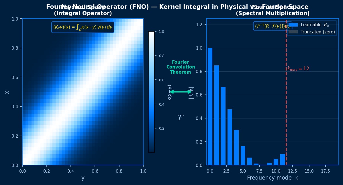
The core of an FNO is the Fourier layer, which applies the following transform to an input field \( v(x) \).
$$ (\mathcal{K} v)(x) = \mathcal{F}^{-1}\!\left( R_\phi \cdot \mathcal{F}(v) \right)(x) $$
That is: (1) FFT into frequency space, (2) multiply only the low-frequency modes (truncated at \( k_{max} \)) by learnable weights \( R_\phi \), (3) inverse FFT back to real space, (4) add a pointwise linear transform and a skip connection — the whole operation being a spectral convolution. Where a convolution sees only local interactions, the Fourier layer expresses global interactions in a single layer, which is what makes it a good match for the solution operator of a PDE, with its Green's-function-like global structure.
What "Discretization Invariance" (Resolution Invariance) Means, and Its Conditions
I've heard that an FNO can run inference at a resolution different from the one it was trained at. Is that really true?
In principle, yes. What gets learned is the set of weights on the truncated frequency modes, and those do not depend on how fine the grid is — which is why "zero-shot super-resolution", training at 64×64 and inferring at 256×256, is possible. But it comes with a condition: the only thing that can be represented is frequency content up to the \( k_{max} \) you trained with. Moving to a finer grid does not suddenly let you resolve high-frequency physics the model never saw during training — thin boundary layers, small eddies. "Being able to change the resolution" and "getting the fine detail right" are separate questions, and confusing them is how verification comes to surprise you.
Training in Practice
Designing the Training Data Is the Biggest Cost
Training an FNO needs several hundred to several thousand "input field to output field" pairs, and since that is training data from CFD, the count is precisely the number of FOM (CFD/FEM) runs you have to pay for. Three points govern the data design. (1) Design of the input distribution — the random distribution used to generate the training data must cover the distribution of inputs (boundary conditions, material distributions, shape parameters) that will actually arrive in operation. (2) Resolution and preprocessing — interpolation onto a uniform grid, and normalization of each channel (zero mean, unit variance). (3) Data augmentation — if the problem has symmetries (rotation, translation, reflection), augmentation buys effective data volume. Training itself is standard, a relative \( L^2 \) loss with Adam, and the hyperparameters start from the number of modes \( k_{max} \) (12 to 32 or so), the channel width, and the number of layers (around 4).
Non-Periodic Boundaries and Unstructured Meshes
The FFT assumes periodicity, so feeding in a non-periodic problem as it stands produces wrap-around artefacts at the boundaries. The standard remedy is domain padding: extend the domain and let the field taper smoothly to zero. Unstructured meshes and complex geometry are the weak point of plain FNO, and the options are (1) interpolation onto a uniform grid (simple, but degraded near boundaries), (2) geo-FNO, which learns a coordinate transform that rectangularizes the computational domain, and (3) the GINO family, which combines a graph neural network. If "complex geometry with an unstructured mesh" is your main battleground, comparing against alternatives to FNO — GNN-based methods, DeepONet — is mandatory.
Verification Discipline — an ML Model Is Also Subject to V&V
A hold-out relative L2 error on its own is not sufficient verification. Make four items standard: (1) error in the quantity of interest (lift, peak temperature — whatever is consumed downstream), (2) conservation checks (residuals of the mass and energy balance, since an FNO does not guarantee conservation), (3) out-of-distribution detection (confirming how far accuracy degrades on inputs outside the training distribution), (4) spectral comparison (quantifying missing high-frequency content through the energy spectrum). Item (2) in particular is the guard against the accident where FNO predictions are fed straight into a downstream analysis and fields that do not balance slip in.
Guidelines for Practical Adoption
The Payback Calculation — Can You Recover the Data-Generation Cost?
The economics of adopting an FNO come down to simple arithmetic. You pay up front with \( N_{train} \) FOM runs (plus the training cost), after which every evaluation is essentially free — so the criterion is whether the number of evaluations in operation is likely to exceed \( N_{train} \) by a wide margin. Shape optimization (thousands of evaluations), Monte Carlo UQ (tens of thousands), and a real-time twin (unbounded) all pay back; a use case that runs a design check a few times a month does not. At a scale that cannot pay back, Kriging (buildable from a few dozen points) is the right answer.
Choosing Among the Surrogate Methods (Recap)
| Method | Data volume | Strength | Uncertainty quantification |
|---|---|---|---|
| Kriging / PCE | Tens to hundreds of points | Parameter dependence of a scalar response | Predictive variance available (Kriging) |
| ROM (POD-based) | Tens to hundreds of snapshots | Dynamic response of a field; embedding in control | Error bounds available (within the RB method) |
| FNO / operator learning | Hundreds to thousands of pairs | Field to field; high input dimensionality (distributions, geometry) | None by default (approximated with ensembles and the like) |
Recommended Adoption Steps
- Reproduce a benchmark — establish the implementation and the training pipeline on a public dataset (Darcy flow, Navier-Stokes, and so on)
- A small version of your own problem — generate a few hundred cases in 2-D with simple geometry and measure the relationship between accuracy and data volume (the learning curve)
- Size the production data volume from the learning curve — extrapolate the \( N_{train} \) needed for the target accuracy before investing in production data generation
- Operation — deploy out-of-distribution detection and an FOM fallback as a set
Implementations and Tools
Implementation Options
| Implementation | Character |
|---|---|
| neuraloperator (PyTorch) | The official library from the original FNO authors. Covers FNO, geo-FNO, and tensor-decomposed variants. Start here |
| NVIDIA PhysicsNeMo | Provides FNO, SFNO and others together with a large-scale training platform. Multi-GPU, industrial use |
| JAX implementations | Research-oriented. Function transforms (vmap/jit) make ablation studies fast |
| Your own PyTorch code | A Fourier layer takes only a few dozen lines. Good for teaching and custom formulations |
Practical Notes on Training and Operation
- Reproducibility — save the seed, the data split, and the normalization constants as deliverables (mismatched normalization constants are the classic production accident)
- Mixed precision — because FFTs are involved, verify that accuracy does not degrade before adopting AMP
- Model size — increasing modes × width × layers hits memory before it causes overfitting. Read the learning curve and start from the smallest configuration
- Version control — record the settings of the FOM used to generate the data (mesh, numerical scheme) as part of the model. If the FOM side changes, retraining is the rule
Research Frontiers
Fusing in Physics Constraints (PINO)
PINO (Physics-Informed Neural Operator), which adds a PDE residual to the FNO loss, is a compromise between the data-driven and physics-constrained approaches. Physics fills in the regions where data is sparse and violations of conservation are suppressed, so research is concentrating on it as the route that targets a reduction in data-generation cost and an improvement in physical consistency at the same time. Because derivatives can be evaluated exactly in Fourier space, the residual computation is also more efficient than in a PINN.
Scaling Up and the "Simulation Foundation Model"
FNO-family models reached accuracy approaching numerical weather prediction at orders-of-magnitude greater speed in weather forecasting (SFNO, the spherical-harmonic version, and FourCastNet), demonstrating that scaling works. That line is developing into the concept of a simulation foundation model: a general-purpose operator pretrained across diverse physics and geometries, then fine-tuned for the individual problem. The implication for CAE practice is that the data requirement may in future fall to "a few hundred cases of your own data plus fine-tuning of a pretrained model".
Generalizing Over Geometry — geo-FNO, GINO, Point-Cloud Methods
The input to practical CAE is very often the geometry itself, so the focus is how to generalize an FNO — which presumes a rectangular grid — over shapes. The options are multiplying rapidly: learned coordinate transforms (geo-FNO), SDF (signed distance field) inputs, composition with graph operators (GINO), and point-cloud transformers. Reports of speed-ups of thousands of times over the FOM keep coming for "geometry to field" problems such as external automotive aerodynamics and aerofoils. As with every other surrogate, designing the distribution of shapes — the diversity of the training geometries — dominates the accuracy.
Troubleshooting
Symptoms, Causes, and Fixes
| Symptom | Likely cause | Fix |
|---|---|---|
| Predicted field is blurred; fine detail disappears | Mode truncation plus the smoothing bias of the L2 loss | Increase k_max; add a spectral or gradient loss; or redefine whether it is good enough judged on the quantity of interest |
| Wave-like artefacts near the boundaries | A non-periodic problem violating the periodicity assumption | Enlarge the domain padding; feed the boundary conditions in as a channel |
| Accuracy drops at high-resolution inference | Over-trusting "discretization invariance" (the spectral limit fixed at training time); degradation from the interpolation preprocessing | Train and verify at several resolutions including the target resolution |
| Hold-out looks good but operation misses | Operational inputs fall outside the training distribution | Redesign the input distribution and retrain. Deploy out-of-distribution detection (reconstruction error and the like) |
| Fields appear that violate conservation | An FNO does not guarantee conservation | Move to PINO; apply a conservative projection to the output (post-processing); make the balance check a gate |
| Training plateaus (the loss stops falling) | Inadequate normalization, insufficient data, error accumulation over time evolution | Check the per-channel normalization; measure the effect of more data on the learning curve; move to rollout training if autoregressive |
How to Answer "How Much Data Do We Need?"
So in the end, how many FOM runs does it take before an FNO is usable? Papers quote things like 1000 cases…
The honest answer is "it depends on the effective dimension of the problem — so measure the learning curve yourself". Plot the hold-out error as you increase the data at N=100, 200, 400 and so on, and the error falls as a power law. Extrapolate that slope and you have an estimate of "the N needed for the target accuracy". Doing that estimate before the real investment in data generation is the crux of budget control on an FNO project. If the slope is too shallow — doubling the data cuts the error by only 20% — then the model or the input representation needs redesigning first, and brute-forcing more data is the wrong move. The learning curve is, for an ML project, the basic verification that corresponds to a mesh convergence study.
Related: PINNs for fluid analysis, reduced order models (ROM), Kriging surrogates.
detail
error