Muffler Design Simulation
Muffler Design: Theoretical Foundations
Overview: Basic Principles of Mufflers
Professor, how do you simulate muffler noise reduction design? Engine exhaust noise is really loud, right?
Good question. Muffler noise reduction design is simulated in two main stages. First, initial design is done using 1D acoustic analysis (Transfer Matrix Method), then detailed shape effects are evaluated with 3D FEM acoustic analysis.
You separate it into 1D and 3D? Why not just do it in 3D from the start?
There are practical reasons. Automotive mufflers are composite types combining 5-10 expansion chambers and resonators to achieve over 30 dB of transmission loss. The combinations of chamber count, pipe diameter, and length are enormous, so first we sweep thousands of patterns in 1D to narrow down promising configurations, then move to 3D. If we started directly with 3D, each case would take several hours, making the design process infeasible.
There are three basic noise reduction mechanisms:
- Reflective Type (Reactive Type): Uses impedance mismatch at expansion chambers to reflect sound waves. Works over a broad band like a low-pass filter.
- Resonant Type: Uses Helmholtz resonators or side branches to eliminate specific frequencies precisely.
- Absorptive Type (Dissipative Type): Converts sound energy into heat using absorbing materials like glass wool.
Actual mufflers are composite types combining these three.
I see, so it's like designing an electrical circuit filter?
Exactly! In fact, acoustic systems and electrical circuits are mathematically equivalent. By mapping sound pressure → voltage, volume velocity → current, and duct impedance → circuit impedance, electrical circuit filter design techniques can be used directly. This correspondence is called acoustic-electrical analogy.
Definition of Transmission Loss (TL)
What's the metric for muffler performance? Something like "how many dB of noise reduction," right?
The most basic metric is Transmission Loss TL. It's the logarithmic ratio of incident acoustic power $W_i$ to transmitted acoustic power $W_t$:
The important point about TL is that it's an intrinsic property of the muffler. It doesn't depend on the sound source or tailpipe radiation conditions, making it easy to use as a design metric in simulation. On the other hand, Insertion Loss IL, which indicates how much the sound is actually reduced, depends on the overall system conditions, so it's used in final vehicle verification.
So the flow is to design with TL and verify with IL, right?
Theory of Expansion Chamber Mufflers
Expansion chamber type, that's where the pipe suddenly gets wider, right? Why does that reduce noise?
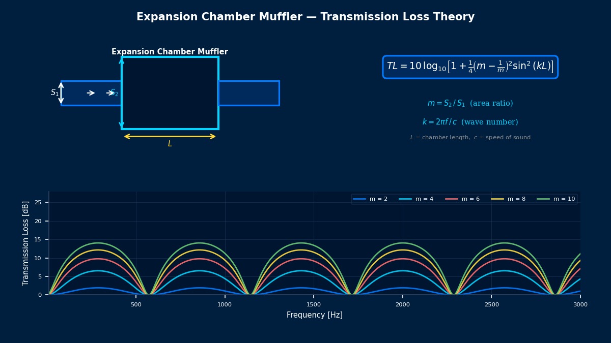
When the duct cross-sectional area changes abruptly, acoustic impedance mismatch occurs, causing part of the sound wave to reflect. If the inlet pipe cross-sectional area is $S_1$, the expansion chamber area is $S_2$, and the chamber length is $L$, then using the area ratio $m = S_2/S_1$, the transmission loss is given by:
Here $k = 2\pi f/c$ is the wavenumber, $f$ is frequency, and $c$ is the speed of sound. Key points from this equation:
- Larger area ratio $m$ increases noise reduction (but also increases back pressure).
- When $\sin^2(kL) = 0$, TL = 0, meaning "pass bands" appear at $f = nc/(2L)$ ($n = 1,2,3,...$) where noise reduction effect is zero.
- Maximum noise reduction occurs when $kL = \pi/2 + n\pi$.
For example, if $m = 9$ (diameter tripled), $L = 0.3$ m, the maximum TL is about 19 dB.
The noise reduction becomes zero at pass bands? That's a problem. How do you handle that?
That's why actual mufflers arrange multiple expansion chambers of different lengths in series. The pass bands of each chamber occur at different frequencies, so they can fill each other's "gaps." This is like a multi-stage band-stop filter in acoustics. For example, connecting two chambers of lengths 0.2 m and 0.3 m in series, their TLs combine (calculated by multiplying transfer matrices, not adding dB), making pass bands less likely to coincide.
Transfer Matrix Method (TMM)
What is the Transfer Matrix Method? I heard it's the core of 1D analysis.
The Transfer Matrix Method (TMM) represents each element of a muffler (straight pipe, expansion chamber, resonator, etc.) with a 2×2 matrix and calculates the overall acoustic characteristics of the system by multiplying them. It relates the inlet side sound pressure $p_1$ and volume velocity $u_1$ to the outlet side $p_2$, $u_2$:
For example, the transfer matrix for a straight pipe of length $L$ and cross-sectional area $S$ is:
If a muffler is connected as straight pipe → expansion chamber → straight pipe → resonator → straight pipe, the overall transfer matrix is the product of each element's matrix:
Assuming the outlet end is an anechoic termination ($p_2/u_2 = \rho c / S_{\text{out}}$), the overall TL is:
Being able to calculate the noise reduction of a complex muffler just by matrix multiplication is really elegant!
Yes, and because it's 1D, the calculation is instant; sweeping frequency from 0 to about 3000 Hz in 0.5 Hz steps takes less than a second. That's why it's optimal for parametric studies in early design. However, it can't capture 3D shape effects (offset pipes, hole patterns in internal baffles, etc.), which is where 3D FEM comes in.
Helmholtz Resonator
Is a Helmholtz resonator the same principle as the "booming" sound when you blow across a bottle's mouth?
Exactly! It's a spring-mass system resonance where the air in the cavity acts as a spring and the air in the neck acts as a mass. The resonance frequency is:
Here $S$ is the neck cross-sectional area, $V$ is the cavity volume, and $L' = L_{\text{neck}} + 0.85d$ ($d$ is neck diameter) is the effective neck length. The end correction $0.85d$ represents the added mass due to acoustic radiation at the neck end.
For example, if the engine's fundamental order is 200 Hz, can you target that specifically?
Yes. For instance, if noise at 100 Hz is a problem at 3000 rpm for the 2nd order component of a 4-cylinder engine, design a Helmholtz resonator with $f_{\text{res}} = 100$ Hz. With $c = 343$ m/s, neck diameter 40 mm ($S = 0.00126$ m$^2$), neck length 50 mm, the required cavity volume is:
A 0.45-liter cavity, about the size of one plastic bottle. If you create a space of this size behind a baffle in the muffler, you can eliminate 100 Hz precisely. However, the noise reduction bandwidth is narrow (typically about ±10-20% of the resonance frequency), so combining it with expansion chambers is necessary for broadband noise reduction.
The transfer matrix for a Helmholtz resonator is expressed as a parallel connection to the main duct as a side branch. Using the resonator impedance $Z_r$:
Absorptive Muffler
How does the type that uses absorbing materials work?
Absorptive mufflers have a structure with glass wool or rock wool packed outside perforated metal. As sound waves pass through the porous material, sound energy is converted to heat by viscous friction and thermal conduction loss. Unlike reflective types, they are characterized by being effective over a broad band in the mid-to-high frequency range.
The Delany-Bazley model is widely used for modeling absorbing materials. From the flow resistivity $\sigma$ (Pa·s/m$^2$), it determines the material's complex speed of sound and complex density as functions of frequency. In simulation, the absorbing material region is treated as an equivalent fluid and coupled with the regular acoustic domain.
I hear sports car mufflers have less glass wool and have a "good sound." Are they deliberately reducing absorption in the design?
Sharp observation. In sports cars, sound design is performed to create a "pleasant engine sound" by deliberately leaving specific frequency bands (sounds corresponding to engine rotation orders). They not only reduce absorption but also actively control the frequency characteristics of exhaust sound through resonator tuning and variable valves. This is also optimized through simulation.
Design Errors Caused by Confusing Transmission Loss (TL) and Insertion Loss (IL)
In practice, it's surprisingly common to confuse the muffler performance metrics TL and IL and use them incorrectly in design. TL is an intrinsic property value of the muffler, independent of source characteristics and radiation end conditions, making it easy to obtain in simulation. IL, on the other hand, is the actual noise reduction when the muffler is installed in a real system, and its value changes significantly depending on the connected engine and exhaust pipe length, even for the same muffler. Complaints like "We calculated 20 dB TL during design, but it only reduced by 8 dB in the actual vehicle" can easily arise if these two are not understood. TL is only the "muffler's capability," and the "effect in the system" must be evaluated with IL.
Computational Methods for Muffler Design
Acoustic Wave Equation and FEM Formulation
When analyzing a muffler with 3D FEM, what equations do you solve?
The foundation is the Helmholtz equation. It's the acoustic wave equation assuming time-harmonic ($e^{j\omega t}$) conditions, solving for the spatial distribution of sound pressure $p$:
Applying the Galerkin method to get the weak form yields the discretized FEM equation:
Here $[K]$ is the acoustic stiffness matrix (spatial integral of pressure gradient), $[M]$ is the acoustic mass matrix (volume integral), and $\{f\}$ is the input source vector. The difference from structural FEM is that the unknown is only the scalar sound pressure. Structures have three displacement components, so for the same number of nodes, acoustic FEM matrices are smaller.
How do you calculate TL from the FEM results?
Incident a unit sound pressure plane wave at the inlet surface and set the outlet surface as an anechoic termination (perfectly matched layer, PML). Separate the incident and reflected waves at the inlet surface, and calculate TL from the acoustic power ratio between the incident wave and the transmitted wave at the outlet surface. Methods called 3-point method or 4-point method are common.
Boundary Element Method (BEM) for External Radiation
Related Topics
Experience the theory with an interactive acoustics and vibration simulator
Acoustic Standing Wave Simulator All Simulators