CFD Analysis of Wind Turbines
CFD Analysis of Wind Turbines: Theoretical Foundations
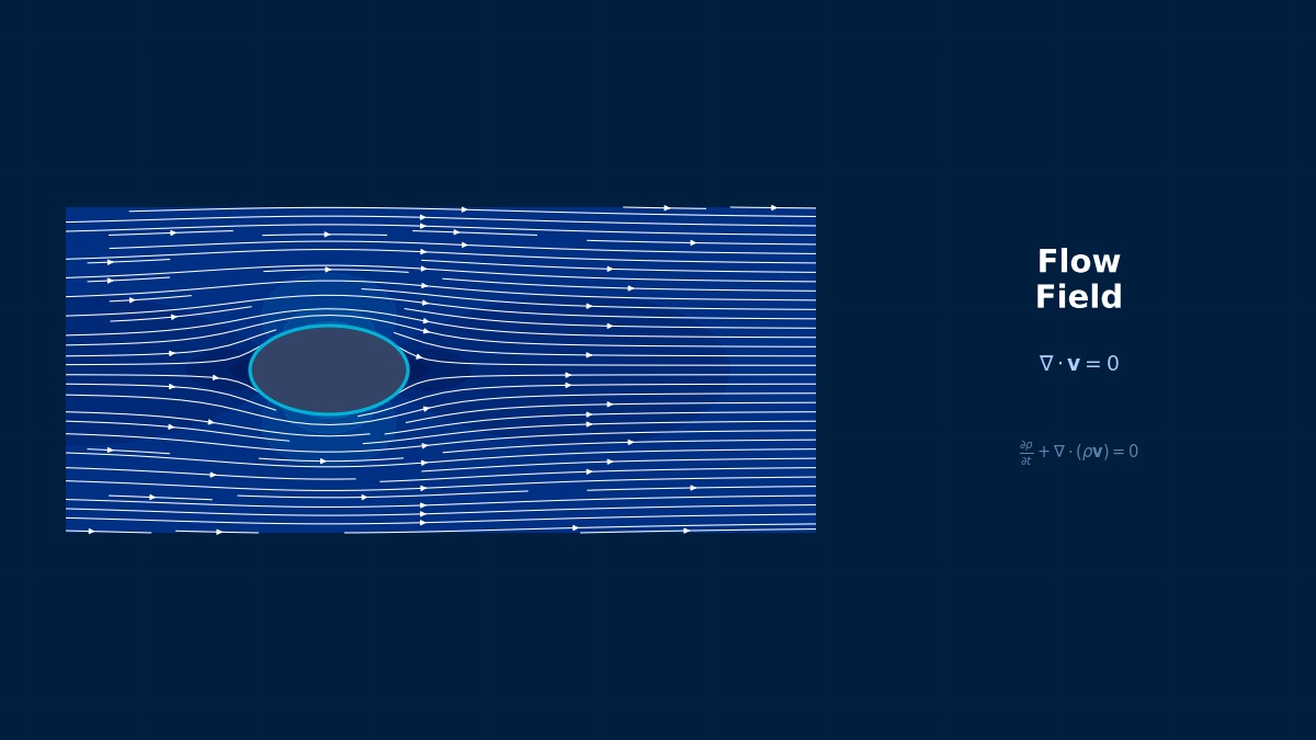
Overview
Professor, how is CFD analysis used for wind turbine blades?
CFD for wind turbines is used for three main purposes: (1) Aerodynamic design of blades and power output prediction, (2) Wake analysis for wind farm layout optimization, and (3) Structural load evaluation under extreme wind conditions.
The theoretical upper limit for wind turbine power output is defined by the Betz limit. The key challenge in blade design is how close one can get to this limit.
Betz Limit and Power Coefficient
Wind turbine power coefficient:
Betz limit (theoretical maximum efficiency):
This is the theoretical upper limit where about 59.3% of the wind's energy can be extracted. The actual $C_P$ for large wind turbines (e.g., Vestas V164, Siemens Gamesa SG 14-222) is around 0.45--0.50, reaching about 80--85% of the Betz limit.
85% is quite close to the theoretical limit.
This is achieved through airfoil design, pitch control, and variable-speed operation optimization. Since there is little room for further improvement here, reducing wake losses across the entire wind farm has become the next focus.
Relationship Between BEM Theory and CFD
Blade Element Momentum theory (BEM) is the foundation of wind turbine analysis.
Here, $a$ is the axial induction factor, $a'$ is the tangential induction factor, and $\omega$ is the rotational angular velocity.
If BEM exists, why is CFD necessary?
BEM has limitations.
| Limitations of BEM | Advantages of CFD |
|---|---|
| Cannot account for 3D effects (root/tip vortices) | Solves 3D flow directly |
| Difficult to predict dynamic stall | Reproducible with unsteady CFD |
| Ignores interference between blades | Analyzes all blades simultaneously |
| Wake model is simplified | Directly calculates wake diffusion/merging |
| Ignores nacelle/tower interference | Reproduces tower shadow |
Tip Speed Ratio and Airfoils
Tip Speed Ratio (TSR):
For large wind turbines, the optimal $\lambda$ is approximately 6--9.
Wind turbine airfoils:
| Airfoil Series | Developer | Characteristics |
|---|---|---|
| NACA 63-xxx | NACA | Classical. Proven track record |
| DU (Delft) | Delft University of Technology | Thick airfoil. Used for root sections |
| FFA-W3 | FOI (Sweden) | High $C_{L,max}$. Insensitive to surface roughness |
| DTU-LN1xx | DTU (Denmark) | Latest design. CFD-optimized |
So the airfoil is different at the root and tip of the blade.
The root section uses thick airfoils (relative thickness 30--40%) for structural strength, while the tip section uses thin airfoils (relative thickness 18--24%) for aerodynamic performance. The airfoil shape changes continuously along the span.
The Reason Blades Are Twisted—Aerodynamic Basis of Pitch Angle
If you look closely at a wind turbine blade, you'll notice it twists from the root to the tip. This design is called "pitch distribution (twist angle)," and the reason is that the direction of the relative wind speed changes at each position. At the tip, the circumferential speed is high, resulting in a small angle of attack relative to the incoming wind, so the twist corrects the angle of attack. The basic task in blade design is to meticulously verify this optimal pitch distribution, derived from Betz theory, using CFD. Every "visually strange shape" has a proper fluid dynamic reason behind it.
Computational Methods for CFD Analysis of Wind Turbines
Analysis Method Hierarchy
What methods are used for wind turbine CFD?
There is a hierarchy of methods based on the trade-off between computational cost and accuracy.
| Method | Modeling | Cell Count | Application |
|---|---|---|---|
| BEM | 1D cross-section theory | -- | Initial design, annual power generation prediction |
| Actuator Disk (AD) | Represents rotor with volume forces | 1 million--10 million | Wind farm layout |
| ALM (Actuator Line) | Distributes volume forces along lines | 5 million--50 million | Wake analysis (LES) |
| Full Blade RANS | Directly solves 3D blade geometry | 10 million--50 million | Blade aerodynamic design |
| Full Blade LES | 3D blade + LES | 100 million--1 billion | Research purposes |
What is the Actuator Line Model (ALM)?
It's a method that does not physically model the blades but distributes volume forces equivalent to lift and drag along rotating lines. Since there's no need to resolve the blade boundary layer, the mesh count can be drastically reduced. It's a standard method for LES of wind farms.
Full Blade CFD Mesh
Full blade analysis for large wind turbines (rotor diameter ~200m class):
- Rotating domain: Cylinder 1.2 times the rotor diameter. Rotates using Sliding Mesh.
- Stationary domain: Outer boundary at least 10 times the rotor diameter.
- Blade surface: $y^+ < 1$, at least 20 prism layers.
- Tip vortex resolution: Refinement zone near the tip.
- Nacelle/Tower: Included in the same mesh (for tower shadow evaluation).
- Total cell count: 5 million--15 million cells per blade.
So for 3 blades + nacelle + tower, it becomes tens of millions of cells.
It's also possible to use a 1/3 model (1 blade + periodic boundary conditions) by exploiting rotational symmetry. However, evaluating tower shadow requires all three blades.
Turbulence Model
Turbulence model selection for wind turbine CFD:
| Model | Application | Notes |
|---|---|---|
| SST k-omega | Blade steady-state aerodynamics | Insufficient for dynamic stall |
| $\gamma$-$Re_\theta$ + SST | Transition prediction (blade root section) | Transition on thick airfoils is important |
| DDES (SST-based) | Dynamic stall, tower shadow | Unsteady calculation mandatory |
| LES (ALM) | Wind farm wake | Atmospheric boundary layer turbulence generation required |
Time Step and Rotation Handling
Time step for unsteady analysis of rotating blades:
For a typical large turbine (rotational speed 12rpm = 0.2rps) at 1 degree per step:
360 steps per revolution. 10 revolutions would be 3600 steps.
The standard practice is to discard at least the first 5 revolutions to exclude the initial transient state, then take a time average over the subsequent 5--10 revolutions.
Why "Time Step is Critical" in CFD for Rotating Blades
When setting up a rotating domain for wind turbine CFD, the time step setting is delicate. The angle the turbine rotates per step is typically kept below 1-2°, which for a rated speed of 15rpm results in a time step of about 0.01-0.02 seconds. If it's too coarse, the generation and transport of tip vortices become inaccurate, leading to large errors in power output prediction. "Saving on time steps makes you cry later" is a classic lesson in wind CFD, and in practice, it's a golden rule to perform a time step sensitivity test along with convergence checks at the outset.
Learn and experience the theory with interactive simulators in this field
All Simulators