Shock Wave-Boundary Layer Interaction
Shock Wave-Boundary Layer Interaction: Theoretical Foundations
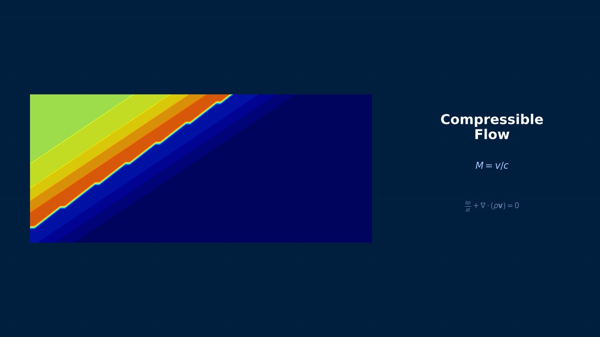
Shock Wave-Boundary Layer Interaction (SBLI)
Professor, Shock Wave-Boundary Layer Interaction (SBLI) is often mentioned in supersonic flow discussions, but what exactly is this phenomenon?
It's a strong interaction that occurs when a shock wave intersects a wall boundary layer in compressible flow. When the sudden pressure rise from the shock wave propagates into the boundary layer, the low-speed fluid within the boundary layer cannot withstand the adverse pressure gradient and separates. This separation bubble and the shock wave mutually influence each other, creating a highly complex flow field.
So separation and shock waves occur together. In what situations does this become a problem?
Typical examples are shock wave/boundary layer interaction inside intakes, separation induced by transonic shocks on wing surfaces, and shock wave reflection within scramjet engines. All of these are directly linked to sudden aerodynamic performance degradation, unsteady loads, or vehicle vibration, making them one of the most critical design issues in the aerospace field.
Governing Equations and Dimensionless Parameters
What equations and metrics are used to describe SBLI?
The foundation is the compressible Navier-Stokes equations, but what's particularly important for SBLI are the relations across the incident shock wave and the separation criterion for the boundary layer. First, the pressure ratio across an oblique shock wave can be expressed as:
$$ \frac{p_2}{p_1} = 1 + \frac{2\gamma}{\gamma+1}(M_1^2 \sin^2\beta - 1) $$
Here, $\beta$ is the shock angle and $M_1$ is the upstream Mach number. This pressure jump acts on the boundary layer.
Does a larger pressure jump make separation more likely?
Exactly. According to Free Interaction Theory, the pressure rise required for separation onset is determined by the upstream boundary layer state. For laminar boundary layers, the required pressure rise for separation is very small, but turbulent boundary layers, due to higher momentum near the wall, are more resistant to separation. The interaction pressure parameter is often used as an indicator of interaction strength.
$$ \chi = \frac{p_{plateau}/p_1 - 1}{(C_f/2)^{1/2}} $$
$C_f$ is the upstream skin friction coefficient. Larger $\chi$ indicates stronger interaction and the formation of larger separation bubbles.
So laminar and turbulent flows are completely different. In real aircraft, the transition location probably also plays a role...
That's precisely the difficulty of SBLI. The shock wave can sometimes induce boundary layer transition, or transition to turbulence may have already occurred upstream of the shock. Shock-Induced Transition is particularly important in scramjet intake design, where the accuracy of transition location prediction directly impacts engine performance estimation.
Classification of Interaction Patterns
Are there different types of SBLI?
Edney's classification is famous, categorizing six types from Type I to Type VI based on the shock wave and boundary layer intersection pattern. Let me introduce some representative ones.
Classification Interaction Pattern Characteristics Real-World Example Type I Oblique Shock/Boundary Layer Most common. Formation of separation bubble. Intake wall surface Type II Shock Wave/Shock Wave/Boundary Layer Supersonic jet impinging on a wall. Jet deflection Type III Normal Shock/Boundary Layer Lambda-type shock structure. Transonic wing surface Type IV Shock Wave/Shock Wave Intersection Supersonic jet formation, extreme heating. Leading edge shape interference
Type IV says 'extreme heating'. How dangerous is it?
Local heat fluxes several to over ten times higher than non-interacting conditions can occur. A famous case is the problem encountered on the Space Shuttle's leading edge. Missing this during the design phase can cause the thermal protection system to fail, so prior prediction using CFD is essential.
Coffee Break Trivia Corner
The Origin of SWBLI Research—Mysterious Separation in 1940s Wind Tunnel Photos
Systematic research on Shock Wave-Boundary Layer Interaction (SWBLI) began in the late 1940s after World War II. Researchers of that era, conducting oil film visualization on supersonic airfoils in wind tunnels, noticed unexpected flow separation patterns appearing at the foot of shock waves. Elucidating the phenomenon of "the boundary layer detaching when a shock wave hits" was an urgent need for supersonic aircraft design. Theories from that era, such as the "Free Interaction Theory" by Lees & Reeves (1956) and Chapman's (1958) separation length correlation, are still used for introductory understanding today. This is a field pioneered with pencils and rulers before numerical computation (CFD) became available.
Professor, Shock Wave-Boundary Layer Interaction (SBLI) is often mentioned in supersonic flow discussions, but what exactly is this phenomenon?
It's a strong interaction that occurs when a shock wave intersects a wall boundary layer in compressible flow. When the sudden pressure rise from the shock wave propagates into the boundary layer, the low-speed fluid within the boundary layer cannot withstand the adverse pressure gradient and separates. This separation bubble and the shock wave mutually influence each other, creating a highly complex flow field.
So separation and shock waves occur together. In what situations does this become a problem?
Typical examples are shock wave/boundary layer interaction inside intakes, separation induced by transonic shocks on wing surfaces, and shock wave reflection within scramjet engines. All of these are directly linked to sudden aerodynamic performance degradation, unsteady loads, or vehicle vibration, making them one of the most critical design issues in the aerospace field.
What equations and metrics are used to describe SBLI?
The foundation is the compressible Navier-Stokes equations, but what's particularly important for SBLI are the relations across the incident shock wave and the separation criterion for the boundary layer. First, the pressure ratio across an oblique shock wave can be expressed as:
Here, $\beta$ is the shock angle and $M_1$ is the upstream Mach number. This pressure jump acts on the boundary layer.
Does a larger pressure jump make separation more likely?
Exactly. According to Free Interaction Theory, the pressure rise required for separation onset is determined by the upstream boundary layer state. For laminar boundary layers, the required pressure rise for separation is very small, but turbulent boundary layers, due to higher momentum near the wall, are more resistant to separation. The interaction pressure parameter is often used as an indicator of interaction strength.
$C_f$ is the upstream skin friction coefficient. Larger $\chi$ indicates stronger interaction and the formation of larger separation bubbles.
So laminar and turbulent flows are completely different. In real aircraft, the transition location probably also plays a role...
That's precisely the difficulty of SBLI. The shock wave can sometimes induce boundary layer transition, or transition to turbulence may have already occurred upstream of the shock. Shock-Induced Transition is particularly important in scramjet intake design, where the accuracy of transition location prediction directly impacts engine performance estimation.
Are there different types of SBLI?
Edney's classification is famous, categorizing six types from Type I to Type VI based on the shock wave and boundary layer intersection pattern. Let me introduce some representative ones.
| Classification | Interaction Pattern | Characteristics | Real-World Example |
|---|---|---|---|
| Type I | Oblique Shock/Boundary Layer | Most common. Formation of separation bubble. | Intake wall surface |
| Type II | Shock Wave/Shock Wave/Boundary Layer | Supersonic jet impinging on a wall. | Jet deflection |
| Type III | Normal Shock/Boundary Layer | Lambda-type shock structure. | Transonic wing surface |
| Type IV | Shock Wave/Shock Wave Intersection | Supersonic jet formation, extreme heating. | Leading edge shape interference |
Type IV says 'extreme heating'. How dangerous is it?
Local heat fluxes several to over ten times higher than non-interacting conditions can occur. A famous case is the problem encountered on the Space Shuttle's leading edge. Missing this during the design phase can cause the thermal protection system to fail, so prior prediction using CFD is essential.
The Origin of SWBLI Research—Mysterious Separation in 1940s Wind Tunnel Photos
Systematic research on Shock Wave-Boundary Layer Interaction (SWBLI) began in the late 1940s after World War II. Researchers of that era, conducting oil film visualization on supersonic airfoils in wind tunnels, noticed unexpected flow separation patterns appearing at the foot of shock waves. Elucidating the phenomenon of "the boundary layer detaching when a shock wave hits" was an urgent need for supersonic aircraft design. Theories from that era, such as the "Free Interaction Theory" by Lees & Reeves (1956) and Chapman's (1958) separation length correlation, are still used for introductory understanding today. This is a field pioneered with pencils and rulers before numerical computation (CFD) became available.
Computational Methods for Shock Wave-Boundary Layer Interaction
Limitations of RANS Analysis and Turbulence Model Selection
When solving SBLI with CFD, how reliable is RANS analysis?
This could be said to be the biggest challenge for CFD of SBLI. RANS turbulence models have difficulty accurately predicting boundary layer behavior under the sudden adverse pressure gradient caused by shock waves. Particularly, the accuracy of separation bubble size and reattachment location becomes problematic.
Do results vary significantly depending on the model?
They vary greatly. The tendencies of representative models are summarized below.
| Turbulence Model | Separation Prediction | Wall Pressure | Heat Flux | Computational Cost |
|---|---|---|---|---|
| SA (Spalart-Allmaras) | Underestimates separation | Slightly inaccurate | Tends to overestimate | Low |
| SST $k$-$\omega$ | Relatively good | Good | Moderate accuracy | Low |
| $k$-$\omega$ GEKO | Parameters adjustable | Depends on adjustment | Depends on adjustment | Low |
| RSM (Reynolds Stress) | Improved but unstable | Good | Slightly improved | Medium |
SST $k$-$\omega$ offers the best practical balance, but for strong interactions, it can still underestimate separation length by 20-30%.
LES/DES for High-Accuracy Analysis
To improve accuracy further, is LES the way to go?
Wall-Resolved LES offers the highest accuracy, but the mesh requirements near the wall are very strict: $\Delta x^+ \sim 50$, $\Delta y^+ < 1$, $\Delta z^+ \sim 20$. For high Re number wall-bounded flows like SBLI problems, the cell count becomes enormous. Therefore, in practice, DES (Detached Eddy Simulation) or WMLES (Wall-Modeled LES) are effective.
What's the difference between DDES and SBES?
DDES uses a shielding function to separate RANS and LES regions, but an ambiguous area called the "Grey Area" tends to appear in the switching zone. SBES is a method that improves this Grey Area problem, making the transition from the RANS stress tensor to the LES stress tensor smoother. It's available in Ansys Fluent 2020R1 and later.
Spatial Discretization Scheme Selection
What numerical scheme should be used to capture shock waves?
Upwind schemes are fundamental for shock wave capturing. Let me show some representative options.
Scheme Characteristics Shock Wave Resolution Numerical Diffusion Roe Approximate Riemann solver. Sharp shock waves. High Moderate AUSM+ Pressure-velocity splitting type. Stable for shocks. High Slightly less HLLC Robust. Also captures contact discontinuities. Medium-High Slightly more Central Differencing + Artificial Viscosity Suitable for LES. Viscosity added only near shocks. Adjustable Low
Related Topics
Fluid Analysis (CFD)Transonic Buffet — Theory and Physical MechanismsGlossaryShock Wave — CAE GlossaryFluid Analysis (CFD)Supersonic Flow — Advanced Topics and Scramjet CFDFluidRadial Turbine — High Expansion Ratio Design and Supersonic FlowFluidAirfoil and Wing Aerodynamic AnalysisFluidCompressor CFD Analysis — Application to Turbocharger Compressors
Related SimulatorsExperience the theory firsthand with the interactive simulator for this field
All Simulators
Rate this articleThank you for your feedback!HelpfulMore detailsReport error
To improve accuracy further, is LES the way to go?
Wall-Resolved LES offers the highest accuracy, but the mesh requirements near the wall are very strict: $\Delta x^+ \sim 50$, $\Delta y^+ < 1$, $\Delta z^+ \sim 20$. For high Re number wall-bounded flows like SBLI problems, the cell count becomes enormous. Therefore, in practice, DES (Detached Eddy Simulation) or WMLES (Wall-Modeled LES) are effective.
What's the difference between DDES and SBES?
DDES uses a shielding function to separate RANS and LES regions, but an ambiguous area called the "Grey Area" tends to appear in the switching zone. SBES is a method that improves this Grey Area problem, making the transition from the RANS stress tensor to the LES stress tensor smoother. It's available in Ansys Fluent 2020R1 and later.
What numerical scheme should be used to capture shock waves?
Upwind schemes are fundamental for shock wave capturing. Let me show some representative options.
| Scheme | Characteristics | Shock Wave Resolution | Numerical Diffusion |
|---|---|---|---|
| Roe | Approximate Riemann solver. Sharp shock waves. | High | Moderate |
| AUSM+ | Pressure-velocity splitting type. Stable for shocks. | High | Slightly less |
| HLLC | Robust. Also captures contact discontinuities. | Medium-High | Slightly more |
| Central Differencing + Artificial Viscosity | Suitable for LES. Viscosity added only near shocks. | Adjustable | Low |
Related Topics
Experience the theory firsthand with the interactive simulator for this field
All Simulators