Eulerian Granular Model
Eulerian Granular: Theoretical Foundations
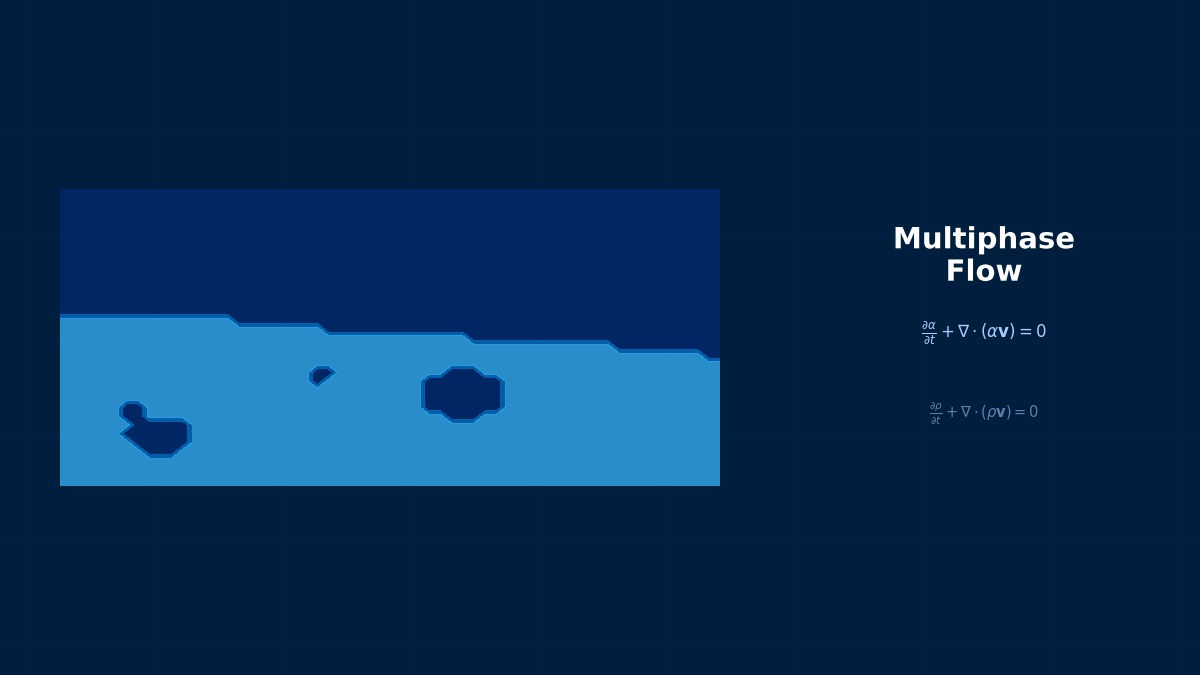
Overview
Professor, what is an Eulerian granular model? Does it treat particles as a continuum?
Exactly. The Eulerian Granular Model treats a collection of powders or granules as a pseudo-continuum called the "granular phase" and solves it together with the gas phase within the Euler-Euler framework. It is widely used for gas-solid two-phase flows such as fluidized beds, pneumatic conveying, cyclones, and powder mixing.
How is it different from DEM-CFD?
DEM-CFD tracks individual particles discretely, but for industrial scales involving millions to billions of particles, the computational cost becomes enormous. The Eulerian granular model treats particle groups as a continuum, allowing solutions for large-scale systems within realistic computation times. However, it cannot directly handle individual particle contact forces or shape effects.
Governing Equations
What are the equations for the granular phase?
To describe the motion of the granular phase, we use KTGF (Kinetic Theory of Granular Flow). The continuity equation for the solid phase is the same as the usual Euler-Euler method, but the characteristic feature is using constitutive relations derived from KTGF for the solid phase stress tensor.
Is KTGF the particle version of the kinetic theory of gases?
Exactly. It characterizes particle velocity fluctuations with the Granular Temperature $\Theta_s$.
The transport equation for Granular Temperature is as follows.
The right-hand side terms are, in order: generation by shear, diffusion ($\kappa_s$ is the diffusion coefficient), dissipation due to inelastic collisions ($\gamma_s$), and gas-solid energy exchange ($\phi_{gs}$).
Solid Phase Constitutive Relations
How are solid phase pressure and viscosity determined?
The solid phase pressure $p_s$ is obtained from Granular Temperature and volume fraction. The model by Lun et al. (1984) is representative.
Here, $e_{ss}$ is the coefficient of restitution between particles, and $g_0$ is the radial distribution function. $g_0$ increases sharply as the volume fraction approaches the maximum packing fraction $\alpha_{s,max}$ (about 0.63), representing contact pressure in densely packed states.
| Constitutive Relation | Model Example | Physical Quantity |
|---|---|---|
| Solid Phase Pressure | Lun, Syamlal-O'Brien | $p_s(\alpha_s, \Theta_s)$ |
| Solid Phase Viscosity | Gidaspow, Syamlal | $\mu_s(\alpha_s, \Theta_s)$ |
| Solid Phase Bulk Viscosity | Lun et al. | $\lambda_s$ |
| Frictional Stress | Schaeffer, Johnson-Jackson | Stress in dense packing region |
The Physics of an Hourglass—Granular Matter is Neither "Fluid" Nor "Solid"
Why does sand in an hourglass appear to "flow," yet remains stationary on a sandpile slope? The Eulerian granular model holds the key to answering this question. Granular matter is a "third state" requiring both hydrodynamic continuum equations and solid-mechanical elastic pressure. The concept of granular temperature is an ingenious idea that treats particle velocity fluctuations as temperature, analogous to molecular thermal motion, derived from the kinetic theory of gases by Jenkins & Richman in the 1980s. Without this theory, it would be difficult to predict even the particle circulation velocity in a CFB boiler within an order of magnitude.
Computational Methods for Eulerian Granular
Details of Numerical Methods
Please tell me the numerical key points of the Eulerian granular model.
The biggest difficulty is handling when the solid volume fraction approaches the maximum packing fraction $\alpha_{s,max}$. In this region, solid phase pressure increases sharply, making it prone to numerical instability.
The Frictional Stress model is important; when $\alpha_s > \alpha_{s,min}$ (typically 0.5), frictional pressure and frictional viscosity are added using the Schaffer model or Johnson & Jackson model.
Drag Model Selection
How should I choose a drag model for gas-solid two-phase flow?
The Gidaspow model is the most common. It switches between the Ergun equation (dense packing region) and the Wen-Yu equation (dilute region) at a volume fraction of 0.8.
| Region | $\alpha_g$ | Model | Equation |
|---|---|---|---|
| Dense Packing | $< 0.8$ | Ergun | $\beta = 150 \frac{\alpha_s^2 \mu_g}{\alpha_g d_s^2} + 1.75 \frac{\alpha_s \rho_g |\mathbf{u}_g - \mathbf{u}_s|}{d_s}$ |
| Dilute | $\geq 0.8$ | Wen-Yu | $\beta = \frac{3}{4} C_D \frac{\alpha_s \alpha_g \rho_g |\mathbf{u}_g - \mathbf{u}_s|}{d_s} \alpha_g^{-2.65}$ |
Doesn't the discontinuity at the switch point cause problems?
Exactly, the discontinuity at the switch point can cause void fraction oscillations. The Huilin-Gidaspow model improves this by introducing a smooth transition function. The Syamlal-O'Brien model also uses a continuous equation across the entire region, offering higher stability.
Implementation in OpenFOAM
Which solver is used in OpenFOAM?
multiphaseEulerFoam supports Eulerian Granular. Each constitutive relation of KTGF can be selected in the kineticTheoryModel class. Main settings are done in constant/phaseProperties.
Settings in Fluent
In Ansys Fluent, enable Granular Phase within the Eulerian Multiphase Model. Important configuration items are as follows.
| Setting | Recommendation | Remarks |
|---|---|---|
| Granular Viscosity | Gidaspow | Standard |
| Granular Bulk Viscosity | Lun et al. | Bulk viscosity |
| Frictional Viscosity | Schaeffer | Dense packing region |
| Packing Limit | 0.63 | Random packing fraction |
| Restitution Coefficient | 0.9 | Typical value for glass beads |
The Wall of KTGF Convergence—The Battle with the "Negative Pressure" Phenomenon
The first stumbling block when implementing an Eulerian granular model is the problem where solid phase pressure becomes negative and diverges. This is a numerical instability that occurs when granular temperature rapidly converges to 0, making setting a floor value (minimum around 1e-10 m²/s²) a de facto essential countermeasure. ANSYS documentation presents the choice of "solving as a Partial Differential Equation or using an Algebraic approximation," but for high-density packing (α_s > 0.4), accuracy often cannot be achieved without the PDE method, requiring on-site judgment of the trade-off between computational cost and accuracy.