Central Difference Scheme
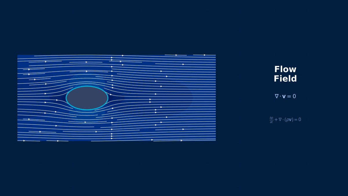
Theory: gradients from both neighbours
Overview
Using central differencing in CFD, I got impossible wiggles in the temperature field. Is it a bug?
Not a bug — a property of central differencing. It computes a gradient from the difference between the two neighbours: second-order accurate, with no artificial diffusion. But when flow (convection) is strong relative to diffusion, the downstream value acts on the node in the wrong direction, and the solution zigzags point to point. The guide is whether the cell Péclet number exceeds 2. Refine the grid or blend in an upwind-type scheme.
Discretised equation
The 1D steady convection–diffusion equation discretised with central differences for both convection and diffusion. The second coefficient on the right turns negative when flow is strong.
Cell Péclet condition
If all coefficients are non-negative, the solution is a weighted average of neighbours and cannot oscillate; that condition is cell Péclet ≤ 2. On the right is the exact solution used below, with global Péclet number $Pe = uL/\Gamma$.
The idea of ‘upwind’
Central-difference oscillation has troubled numerical analysts since the 1950s. In 1952 Courant, Isaacson and Rees proposed differencing with upstream (upwind) values, where information comes from, and the trade — no oscillation, but only first-order accuracy — became known. In the 1980s Harten formalised the conditions for non-oscillatory schemes (TVD), and limited schemes that lean upwind only where changes are steep spread widely. The convection-scheme options in today's general-purpose CFD rest on this long debate.
Worked example: 1D convection–diffusion
Steady convection–diffusion on [0, 1] with 0 at the left, 1 at the right and global Péclet 50, solved with central differencing (CDS) and first-order upwinding (UDS). The exact solution rises steeply near the right end:
| Cells | Cell Pe | CDS minimum | CDS max error | UDS max error |
|---|---|---|---|---|
| 10 | 5.0 | −0.429 | 0.436 | 0.160 |
| 20 | 2.5 | −0.111 | 0.193 | 0.204 |
| 25 | 2.0 | 0.000 | 0.135 | 0.198 |
| 50 | 1.0 | 0.000 | 0.035 | 0.132 |
| 100 | 0.5 | 0.000 | 0.008 | 0.077 |
| 200 | 0.25 | 0.000 | 0.002 | 0.042 |
At 10 cells, the non-oscillating upwind scheme has the smaller error.
Right. On a coarse grid, central differencing drives a solution that should stay between 0 and 1 down to −0.43 — like a temperature below absolute zero, physically impossible. But from 25 cells, where cell Péclet reaches 2, the oscillation disappears and error falls with the square of spacing. At 100 cells central gives 0.008 and upwind 0.077 — a factor of ten. Upwind is first order, so refinement shrinks its error only slowly. It's a trade between ‘stable but crude’ and ‘accurate but conditional’.
Example 2: order of convergence
At Péclet 10 with refinement, central differencing's observed order approached 2.00 and upwinding's 0.97 (at 200 cells, 0.0001 versus 0.0090).
Choosing a scheme
- Estimate the cell Péclet distribution from velocity, spacing and diffusivity (viscosity).
- For steady RANS, default to second-order upwind-type or limited schemes.
- In LES, numerical diffusion damps turbulent eddies, so use central-type schemes (blending a little upwind if needed).
- For steep changes (shocks, thin layers) use limiters that suppress oscillation.
- Refine the grid and confirm results don't change.
“The clean result was wrong”
A CFD study of mixing in a pipe gave a clean, non-oscillating concentration field, yet mixing progressed far faster than in the experiment. First-order upwinding had been used for stability, and numerical diffusion was several times the real diffusion. Switching to a second-order scheme reproduced the slower mixing seen experimentally. A non-oscillating result looks reassuring, but numerical diffusion may be over-mixing. The cruder the upwind result, the more it needs checking with grid refinement.
Common mistakes
Mistakes and fixes
| Mistake | Effect | Fix |
|---|---|---|
| Central differencing on coarse grids | Oscillation, out-of-range values | Keep cell Péclet ≤ 2 |
| Staying first-order upwind | Over-mixing by numerical diffusion | Second-order schemes |
| Upwinding in LES | Eddies damped | Central-type schemes |
| Mistaking oscillation for physics | Wrong conclusions | Check with other grids |
| No oscillation, so correct | Numerical diffusion missed | Check grid convergence |
I'd like to learn related topics.
Try convergence order with the Richardson extrapolation tool. For scheme comparisons see upwind schemes; basics, finite volume fundamentals; time direction, time integration in CFD; high-accuracy methods, spectral methods; and pressure solution, the coupled pressure–velocity solver.
Related Topics
Experience the theory firsthand with the interactive simulator for this field
All Simulators