Euler Buckling Analysis
Euler Buckling: Theoretical Foundations
What is Buckling?
Derivation of the Governing Equation
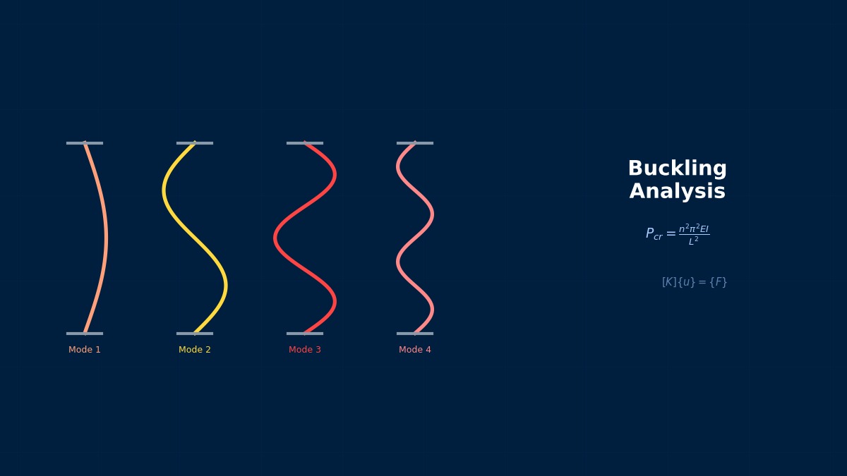
This is the famous Euler buckling load. $n = 2, 3, \ldots$ are higher-order modes, but in real structures, the lowest-order mode ($n=1$, a half-sine wave) is dominant.
Boundary Conditions and Effective Buckling Length
| Boundary Condition | K Value | $P_{cr}$ Ratio | Practical Example |
|---|---|---|---|
| Both ends pinned | 1.0 | 1.0 (reference) | Idealized truss members |
| One end fixed, one end free (cantilever) | 2.0 | 0.25 | Flagpoles, free-standing columns |
| Both ends fixed | 0.5 | 4.0 | Columns between concrete walls |
| One end fixed, one end pinned | 0.7 | 2.04 | Steel frame columns with fixed base and beam connections |
Slenderness Ratio and Applicable Range
Here, $r = \sqrt{I/A}$ is the radius of gyration of the cross-section, and $KL/r$ is the slenderness ratio. The larger the slenderness ratio, the lower $\sigma_{cr}$ becomes — meaning slender columns are more prone to buckling.
For steel ($E = 200$ GPa, $\sigma_Y = 250$ MPa), this is approximately $KL/r > 89$. For "intermediate columns" with a slenderness ratio smaller than this, Johnson's parabolic formula or tangent modulus theory must be used.
Effect of Initial Imperfections
- Buckling Mode Method — Scaling the first mode shape from linear buckling analysis to a small amplitude (about $L/1000$ of the member length) and applying it as the initial shape.
- Design Code Method — Directly reflecting imperfection patterns based on fabrication tolerances (e.g., AIJ's $L/1000$, Eurocode's $L/500$) onto the geometry.
In Abaqus, you can easily incorporate the first mode as an initial imperfection with just the *IMPERFECTION keyword.
Theory Summary
- Buckling is a stability problem, not material failure — A geometric instability phenomenon that occurs within the elastic range.
- $P_{cr} = \pi^2 EI / (KL)^2$ — Boundary conditions (the $K$ value) govern the buckling load.
- The applicable range is determined by the slenderness ratio — Using the Euler formula for short columns leads to a dangerous overestimation.
- Initial imperfections greatly influence real behavior — You must not blindly trust the theoretical $P_{cr}$ value for a perfect column.
Euler's Genius and the Birth of Buckling Theory
The buckling load formula $P_{cr}=\pi^2 EI/(KL)^2$ published by Leonhard Euler in 1744 astonished scholars of the time. No one had anticipated that "the critical load depends entirely on the cross-sectional shape ($I$) and length ($L$), and not at all on the material strength." It is said that even Euler himself lacked confidence in the practical utility of this formula, yet it has been used continuously for over 270 years as the foundation for slender column design.
Computational Methods for Euler Buckling
FEM Formulation for Buckling Analysis
Here, $[K]$ is the usual elastic stiffness matrix, $[K_\sigma]$ is the geometric stiffness matrix (stress stiffness matrix), $\lambda$ is the buckling load factor, and $\{\phi\}$ is the buckling mode shape.
Construction of the Geometric Stiffness Matrix
- Step 1: Perform a linear static analysis under a reference load $F_{ref}$ to obtain the stress state $\sigma_0 = \{\sigma_{xx}, \sigma_{yy}, \sigma_{xy}, \ldots\}$ at each element.
- Step 2: For each element, compute the element-level geometric stiffness matrix $[k_{\sigma,e}]$ from the membrane stress (in-plane stress). For a 2D element, the contribution is: $$[k_{\sigma,e}] = \int_{\Omega_e} [B_L]^T [\sigma_0] [B_L] \, d\Omega$$ where $[B_L]$ is the linear part of the strain-displacement matrix.
- Step 3: Assemble all element matrices into the global geometric stiffness matrix $[K_\sigma]$.
The key insight is: compressive stress reduces stiffness, while tensile stress increases it. This is why buckling occurs primarily in compression.
- Unit load method: Apply $F_{ref} = 1$ N and compute $\lambda$. Then $P_{cr} = \lambda \times 1 = \lambda$.
- Design load method: Apply $F_{ref}$ equal to the expected operating load, and the buckling factor $\lambda$ directly tells you the margin ($\lambda = 2$ means the structure can withstand twice the design load before buckling).
In Nastran (SOL 105) and Abaqus (*BUCKLE), the solver automatically scales the computed eigenvalues $\lambda$ based on the reference load. For Ansys, you typically inspect the eigenvalue multiplier directly.
- Your solver is explicitly running a buckling analysis (not a modal analysis).
- The reference load step is properly defined to generate the geometric stiffness matrix.
- For nonlinear buckling (Riks method), the geometric nonlinearity is enabled.
Related Topics
Experience the theory interactively with a simulator that calculates the critical load for Euler buckling
Euler Buckling Simulator Structural Analysis Tools