熱疲労
Theory and Physics
What is Thermal Fatigue?
Professor, what is thermal fatigue?
Fatigue due to repeated temperature changes. Temperature change → thermal stress → repetition → fatigue failure. A problem in engine cylinder heads, exhaust manifolds, turbine blades, and nuclear piping.
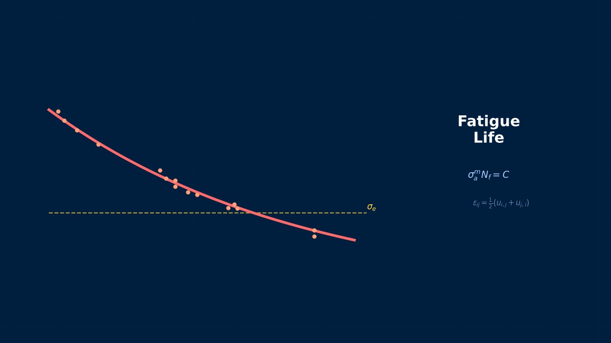
Characteristics of Thermal Fatigue
Summary
Jet Engine Blade Cooling Hole Cracks
Thermal fatigue is fatigue caused by repeated thermal strain due to temperature changes. In the turbine blades of RR's Trent engine, temperatures fluctuate from 900°C during operation to room temperature when stopped, with thermal strain range around cooling holes reaching 0.5%. According to the Coffin-Manson law, this strain range predicts a material life of 5000 to 10000 cycles, forming the basis for major overhauls (C-check).
Physical Meaning of Each Term
- Inertia term (mass term): $\rho \ddot{u}$, meaning "mass × acceleration". Have you ever experienced being thrown forward when slamming on the brakes? That "feeling of being carried away" is precisely the inertial force. Heavier objects are harder to set in motion and harder to stop once moving. Buildings shake during earthquakes because the ground moves suddenly while the building's mass is "left behind". In static analysis, this term is set to zero, assuming "forces are applied slowly so acceleration can be ignored". It absolutely cannot be omitted for impact loads or vibration problems.
- Stiffness term (elastic restoring force): $Ku$ or $\nabla \cdot \sigma$. When you stretch a spring, you feel a "force trying to return it", right? That's Hooke's law $F=kx$, the essence of the stiffness term. Now a question—an iron rod and a rubber band, which stretches more under the same force? Obviously the rubber. This "resistance to stretching" is Young's modulus $E$, which determines stiffness. A common misconception: "high stiffness ≠ strong". Stiffness is "resistance to deformation", strength is "resistance to failure"—different concepts.
- External force term (load term): Body force $f_b$ (gravity, etc.) and surface force $f_s$ (pressure, contact force, etc.). Think of it this way—the weight of a truck on a bridge is a "force acting on the entire interior" (body force), while the force of the tires pushing on the road surface is a "force acting only on the surface" (surface force). Wind pressure, water pressure, bolt tightening force... all are external forces. A common mistake here: getting the load direction wrong. Intending "tension" but ending up with "compression"—sounds like a joke, but it actually happens when coordinate systems are rotated in 3D space.
- Damping term: Rayleigh damping $C\dot{u} = (\alpha M + \beta K)\dot{u}$. Try plucking a guitar string. Does the sound continue forever? No, it gradually fades, right? Because vibration energy is converted to heat by air resistance and internal friction in the string. Car shock absorbers work on the same principle—deliberately absorbing vibration energy to improve ride comfort. If damping were zero? Buildings would keep shaking forever after an earthquake. Since that doesn't happen in reality, setting appropriate damping is crucial.
Assumptions and Applicability Limits
- Continuum assumption: Treats material as a continuous medium, ignoring microscopic heterogeneity
- Small deformation assumption (for linear analysis): Deformation is sufficiently small compared to initial dimensions, stress-strain relationship is linear
- Isotropic material (unless specified otherwise): Material properties are independent of direction (anisotropic materials require separate tensor definition)
- Quasi-static assumption (for static analysis): Ignores inertial and damping forces, considers only balance between external and internal forces
- Non-applicable cases: Large deformation/large rotation problems require geometric nonlinearity. Nonlinear material behavior like plasticity and creep requires constitutive law extension
Dimensional Analysis and Unit Systems
| Variable | SI Unit | Notes / Conversion Memo |
|---|---|---|
| Displacement $u$ | m (meter) | When inputting in mm, unify loads and elastic modulus to MPa/N system |
| Stress $\sigma$ | Pa (Pascal) = N/m² | MPa = 10⁶ Pa. Note unit inconsistency when comparing with yield stress |
| Strain $\varepsilon$ | Dimensionless (m/m) | Note distinction between engineering strain and logarithmic strain (for large deformation) |
| Elastic modulus $E$ | Pa | Steel: ~210 GPa, Aluminum: ~70 GPa. Note temperature dependence |
| Density $\rho$ | kg/m³ | In mm system: tonne/mm³ (= 10⁻⁹ tonne/mm³ for steel) |
| Force $F$ | N (Newton) | Unify as N in mm system, N in m system |
Numerical Methods and Implementation
FEM for Thermal Fatigue
1. Thermal Analysis — Calculate time history of temperature distribution
2. Thermal-Structural Coupling — Temperature distribution → thermal stress → Elastoplastic analysis (Chaboche model recommended)
3. Obtain Stabilized Hysteresis Loop — Stable cycle of stress-strain
4. Fatigue Evaluation — Coffin-Manson + creep damage (summed using Miner's rule)
Summary
Choosing Between Isothermal vs. Non-Isothermal Fatigue Curves
Using isothermal fatigue data as-is for thermal fatigue design carries risk. IN718 nickel superalloy shows 40% shorter life in TMF tests at 400-800°C compared to isothermal tests at 600°C. In analysis, one must decide whether to correct isothermal SN/EN curves by multiplying by a "TMF factor" of 0.5-0.7 or to obtain dedicated TMF fatigue curves. The correction factor method is often used for early-stage development due to cost-effectiveness.
Linear Elements (1st-order elements)
Linear interpolation between nodes. Low computational cost but low stress accuracy. Beware of shear locking (mitigated with reduced integration or B-bar method).
Quadratic Elements (with mid-side nodes)
Can represent curved deformation. Stress accuracy improves significantly, but degrees of freedom increase by about 2-3 times. Recommended: when stress evaluation is critical.
Full Integration vs Reduced Integration
Full Integration: Risk of over-constraint (locking). Reduced Integration: Risk of hourglass modes (zero-energy modes). Choose appropriately for the situation.
Adaptive Mesh
Automatic refinement based on error indicators (e.g., ZZ estimator). Efficiently improves accuracy in stress concentration areas. Includes h-method (element subdivision) and p-method (order increase).
Newton-Raphson Method
Standard method for nonlinear analysis. Updates tangent stiffness matrix each iteration. Quadratic convergence within convergence radius, but high computational cost.
Modified Newton-Raphson Method
Updates tangent stiffness matrix using initial value or every few iterations. Lower cost per iteration but linear convergence speed.
Convergence Criteria
Force residual norm: $||R|| / ||F_{ext}|| < \epsilon$ (typically $\epsilon = 10^{-3}$ to $10^{-6}$). Displacement increment norm: $||\Delta u|| / ||u|| < \epsilon$. Energy norm: $\Delta u \cdot R < \epsilon$
Load Increment Method
Applies full load in small increments rather than all at once. Arc-length method (Riks method) can trace beyond extremum points on the load-displacement curve.
Analogy: Direct Method vs. Iterative Method
The direct method is like "solving simultaneous equations accurately with pen and paper"—reliable but takes too long for large-scale problems. The iterative method is like "repeatedly guessing to approach the correct answer"—starts with a rough answer but improves accuracy with each iteration. It's the same principle as looking up a word in a dictionary: more efficient to open it at an estimated location and adjust forward/backward (iterative) than to search sequentially from the first page (direct).
Relationship Between Mesh Order and Accuracy
1st-order elements are like "approximating a curve with a ruler"—represented by straight line segments, so accuracy is limited. 2nd-order elements are like "flexible curves"—can represent curved changes, dramatically improving accuracy even at the same mesh density. However, computational cost per element increases, so judge based on total cost-effectiveness.
Practical Guide
Thermal Fatigue in Practice
Engine components (cylinder heads, exhaust systems), turbines, nuclear piping.
Practical Checklist
Thermal Fatigue Design of Exhaust Manifolds
Gasoline engine exhaust manifolds are a typical thermal fatigue environment, cycling from 200°C to 900°C from startup to shutdown. For FEM thermal fatigue analysis of SiMo ductile cast iron manifolds, the flow of fluctuating temperature field → thermal strain → elastoplastic stress → strain-life evaluation is essential. Toyota standardized this flow as a design tool from the late 1990s.
Analogy for Analysis Flow
The analysis flow is actually very similar to cooking. First, buy ingredients (prepare CAD model), do prep work (mesh generation), apply heat (solver execution), and finally plate it (visualization in post-processing). Here's an important question—in cooking, which step is most prone to failure? Actually, it's "prep work". If mesh quality is poor, results will be a mess no matter how good the solver is.
Pitfalls Beginners Often Fall Into
Are you checking mesh convergence? Do you think "calculation ran = results are correct"? This is actually the most common trap for CAE beginners. The solver will always return "some answer" for the given mesh. But if the mesh is too coarse, that answer will be far from reality. Confirm that results stabilize with at least three levels of mesh density—neglecting this leads to the dangerous assumption that "the computer gave the answer, so it must be correct".
Thinking About Boundary Conditions
Setting boundary conditions is like "writing the problem statement" for an exam. If the problem statement is wrong? No matter how accurately you calculate, the answer will be wrong. "Is this surface really fully fixed?" "Is this load really uniformly distributed?"—Correctly modeling real-world constraint conditions is actually the most important step in the entire analysis.
Software Comparison
Tools
Practical Flow for Abaqus Thermal Fatigue Coupled Analysis
Abaqus has an established three-step flow: heat transfer analysis (Step 1) → thermal stress analysis (Step 2) → fatigue evaluation (integrated with fe-safe). Through collaboration between DASSAULT and HBM, it's possible to launch fe-safe directly from Abaqus CAE and perform TMF fatigue evaluation including temperature history. Renault improved thermal fatigue life prediction accuracy for turbocharger housings to within ±20% using this flow.
Three Most Important Questions for Selection
- "What are you solving?": Does it support the physical models/element types needed for thermal fatigue? For example, presence of LES support for fluids, contact/large deformation capability for structures makes a difference.
- "Who will use it?": For beginner teams, tools with rich GUI are suitable; for experienced users, flexible script-driven tools are better. Similar to the difference between automatic (GUI) and manual (script) transmission cars.
- "How far will it expand?": Selection considering future analysis scale expansion (HPC support), deployment to other departments, and integration with other tools leads to long-term cost reduction.
Advanced Technologies
Advanced Topics in Thermal Fatigue
Related Topics
なった
詳しく
報告