Chaboche Nonlinear Kinematic Hardening Model
Theory and Physics
What is the Chaboche Model?
Professor, is the Chaboche model the "main contender" for kinematic hardening?
Yes. The Chaboche model is a nonlinear kinematic hardening model and is the most widely used for analyzing cyclic plasticity (low-cycle fatigue, ratcheting, shakedown).
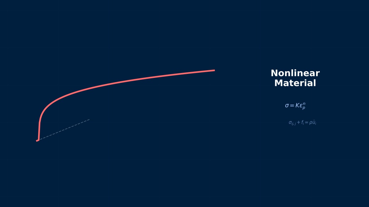
Nonlinear Kinematic Hardening Equation
Evolution law for back stress $\alpha$:
The first term is Prager's linear hardening (forward term), the second term is the dynamic recovery term (which "pulls back" the back stress via $\gamma \alpha$).
So the dynamic recovery term makes it "nonlinear". The back stress saturates at large strains.
$C/\gamma$ is the saturation value of the back stress. $C$ is the initial hardening rate, $\gamma$ is the speed of saturation. In practice, multiple backstresses are superposed ($N = 2 \sim 4$ terms):
Parameter Determination
$C_k, \gamma_k$ are determined from the stabilized hysteresis loop of a repeated tension-compression test (strain-controlled cyclic test). In Abaqus, define the isotropic hardening part with *CYCLIC HARDENING, and use *PLASTIC, HARDENING=COMBINED for combined hardening.
Summary
Key Points:
- $d\alpha = (2/3)C d\varepsilon^p - \gamma \alpha dp$ — Forward + dynamic recovery
- Superposition of multiple backstresses ($N = 2 \sim 4$) — Accurate over a wide stress range
- Determine $C_k, \gamma_k$ from cyclic tests
- Standard model for low-cycle fatigue, ratcheting, shakedown
- Abaqus *PLASTIC, HARDENING=COMBINED — Combined isotropic + kinematic hardening
Chaboche's Background: French Nuclear Power
Jean-Louis Chaboche was affiliated with the French National Aerospace Research Institute (ONERA) and the Atomic Energy Commission (CEA) in the 1970s-80s and developed this model to solve thermal fatigue problems in nuclear reactor piping. The background was France's aggressive nuclear power promotion policy in the 1970s, and the rapidly increasing demand for "engineer-usable cyclic plasticity models" at the time drove the development.
Physical Meaning of Each Term
- Inertia term (mass term): $\rho \ddot{u}$, i.e., "mass × acceleration". Have you ever experienced being thrown forward when braking suddenly? That "feeling of being carried away" is precisely the inertia force. Heavier objects are harder to set in motion and harder to stop once moving. Buildings shake during earthquakes because the ground moves suddenly while the building's mass is "left behind". In static analysis, this term is set to zero, which assumes "forces are applied slowly so acceleration can be ignored". It absolutely cannot be omitted for impact loads or vibration problems.
- Stiffness term (elastic restoring force): $Ku$ or $\nabla \cdot \sigma$. When you pull a spring, you feel a "force trying to return", right? That's Hooke's law $F=kx$, the essence of the stiffness term. Now a question——an iron rod and a rubber band, which stretches more when pulled with the same force? Obviously the rubber. This "resistance to stretching" is the Young's modulus $E$, which determines stiffness. A common misconception: "high stiffness = strong" is incorrect. Stiffness is "resistance to deformation", strength is "resistance to failure" – different concepts.
- External force term (load term): Body force $f_b$ (gravity, etc.) and surface force $f_s$ (pressure, contact force, etc.). Think of it this way——the weight of a truck on a bridge is a "force acting on the entire contents" (body force), the force of the tires pushing on the road surface is a "force acting only on the surface" (surface force). Wind pressure, water pressure, bolt tightening force... all are external forces. A common pitfall here: getting the load direction wrong. Intending "tension" but it becomes "compression"——sounds like a joke, but it actually happens when coordinate systems are rotated in 3D space.
- Damping term: Rayleigh damping $C\dot{u} = (\alpha M + \beta K)\dot{u}$. Try plucking a guitar string. Does the sound continue forever? No, it gradually fades away. That's because the vibration energy is converted to heat by air resistance and internal friction in the string. Car shock absorbers work on the same principle——they intentionally absorb vibration energy to improve ride comfort. What if damping were zero? Buildings would keep shaking forever after an earthquake. Since that doesn't happen in reality, setting appropriate damping is crucial.
Assumptions and Applicability Limits
- Continuum assumption: Treats material as a continuous medium, ignoring microscopic inhomogeneities.
- Small deformation assumption (for linear analysis): Deformation is sufficiently small compared to initial dimensions, and the stress-strain relationship is linear.
- Isotropic material (unless otherwise specified): Material properties are independent of direction (anisotropic materials require separate tensor definitions).
- Quasi-static assumption (for static analysis): Ignores inertia and damping forces, considering only the balance between external and internal forces.
- Non-applicable cases: Large deformation/large rotation problems require geometric nonlinearity. Nonlinear material behavior like plasticity and creep requires constitutive law extensions.
Dimensional Analysis and Unit Systems
| Variable | SI Unit | Notes / Conversion Memo |
|---|---|---|
| Displacement $u$ | m (meter) | When inputting in mm, unify loads and elastic modulus to MPa/N system. |
| Stress $\sigma$ | Pa (Pascal) = N/m² | MPa = 10⁶ Pa. Be careful of unit system inconsistency when comparing with yield stress. |
| Strain $\varepsilon$ | Dimensionless (m/m) | Note the distinction between engineering strain and logarithmic strain (for large deformations). |
| Elastic modulus $E$ | Pa | Steel: ~210 GPa, Aluminum: ~70 GPa. Note temperature dependence. |
| Density $\rho$ | kg/m³ | In mm system: tonne/mm³ (= 10⁻⁹ tonne/mm³ for steel). |
| Force $F$ | N (Newton) | Unify as N in mm system, N in m system. |
Numerical Methods and Implementation
FEM Settings for Chaboche
```
*MATERIAL, NAME=steel_cyclic
*ELASTIC
200000., 0.3
*PLASTIC, HARDENING=COMBINED, NUMBER BACKSTRESSES=3
250., 0.0
*CYCLIC HARDENING
250., 0.0
280., 0.1
300., 0.5
```
NUMBER BACKSTRESSES=3 specifies a 3-term Chaboche model. $C_k, \gamma_k$ can be automatically fitted by Abaqus from stabilized loop data (*PLASTIC, TEST DATA INPUT).
Summary
The Ingenuity of 2-Backstress Superposition
The accuracy of the Chaboche model is determined by the number of backstress terms. In practice, superposition of 2-3 terms is common, with a role division where the first term handles stress saturation in the large strain region, and the second term handles transient hardening. In Chaboche's own 1989 paper, a 3-term model was shown to match isothermal fatigue tests on 304 stainless steel within a 0.3% error.
Linear Elements (1st-order elements)
Linear interpolation between nodes. Low computational cost but low stress accuracy. Beware of shear locking (mitigated with reduced integration or B-bar method).
Quadratic Elements (with mid-side nodes)
Can represent curved deformation. Stress accuracy improves significantly, but degrees of freedom increase by about 2-3 times. Recommended: when stress evaluation is important.
Full integration vs Reduced integration
Full integration: Risk of over-constraint (locking). Reduced integration: Risk of hourglass modes (zero-energy modes). Choose appropriately for the situation.
Adaptive Mesh
Automatic refinement based on error indicators (e.g., ZZ estimator). Efficiently improves accuracy in stress concentration areas. There are h-method (element subdivision) and p-method (order increase).
Newton-Raphson Method
Standard method for nonlinear analysis. Updates the tangent stiffness matrix every iteration. Shows quadratic convergence within the convergence radius, but computational cost is high.
Modified Newton-Raphson Method
Updates the tangent stiffness matrix using the initial value or every few iterations. Cost per iteration is low, but convergence speed is linear.
Convergence Criteria
Force residual norm: $||R|| / ||F_{ext}|| < \epsilon$ (typically $\epsilon = 10^{-3}$〜$10^{-6}$). Displacement increment norm: $||\Delta u|| / ||u|| < \epsilon$. Energy norm: $\Delta u \cdot R < \epsilon$
Load Increment Method
Applies the full load not all at once, but in small increments. The arc-length method (Riks method) can track beyond limit points on the load-displacement curve.
Analogy: Direct Method vs Iterative Method
The direct method is like "solving simultaneous equations accurately with pen and paper"——reliable but takes too long for large-scale problems. The iterative method is like "repeatedly guessing to approach the correct answer"——starts with a rough answer but improves accuracy with each iteration. It's the same principle as looking up a word in a dictionary: opening to an estimated page and adjusting forward/backward (iterative method) is more efficient than searching sequentially from the first page (direct method).
Relationship Between Mesh Order and Accuracy
1st-order elements are like "approximating a curve with a ruler"——represented by straight line segments, so accuracy is limited. 2nd-order elements are like "flexible curves"——can represent curved changes, dramatically improving accuracy even at the same mesh density. However, computational cost per element increases, so judge based on total cost-effectiveness.
Practical Guide
Chaboche in Practice
Used for thermal fatigue in high-temperature nuclear piping, thermal fatigue in automotive engine components, and low-cycle fatigue in aircraft engine turbine disks.
Practical Checklist
Turbine Blade Life Prediction
In the design of CFM56 engine (for Airbus A320) turbine blades, thermo-elasto-plastic cycle analysis using the Chaboche model has been conducted since the 1990s. By analyzing the plastic strain range at the blade root subjected to temperature fluctuations of about 600~1,050℃ per takeoff/landing cycle and evaluating low-cycle fatigue life combined with the Manson-Coffin rule, an overhaul interval of over 30,000 hours was achieved.
Analogy for Analysis Flow
The analysis flow is actually very similar to cooking. First, buy ingredients (prepare CAD model), do the prep work (mesh generation), put it on the heat (solver execution), and finally plate it (post-processing visualization). Here's an important question——which step in cooking is most prone to failure? Actually, it's the "prep work". If mesh quality is poor, no matter how excellent the solver, the results will be a mess.
Pitfalls Beginners Often Fall Into
Are you checking mesh convergence? Do you think "the calculation ran = the result is correct"? This is actually the most common trap for CAE beginners. The solver will always return "some answer" for the given mesh. But if the mesh is too coarse, that answer will be far from reality. Confirm that results stabilize with at least three levels of mesh density——neglecting this leads to the dangerous assumption that "the computer gave the answer, so it must be correct".
Thinking About Boundary Conditions
Setting boundary conditions is the same as "writing the exam question". If the question is wrong? No matter how accurately you calculate, the answer will be wrong. "Is this surface really fully fixed?" "Is this load really uniformly distributed?"——Correctly modeling real-world constraint conditions is actually the most important step in the entire analysis.
Software Comparison
Tools for Chaboche
Selection Guide
Related Topics
なった
詳しく
報告