Level Set Method Topology Optimization

Category: 構造解析 | Integrated 2026-04-06
CAE visualization for topology level set theory - technical simulation diagram
レベルセット法トポロジー最適化

Theory and Physics

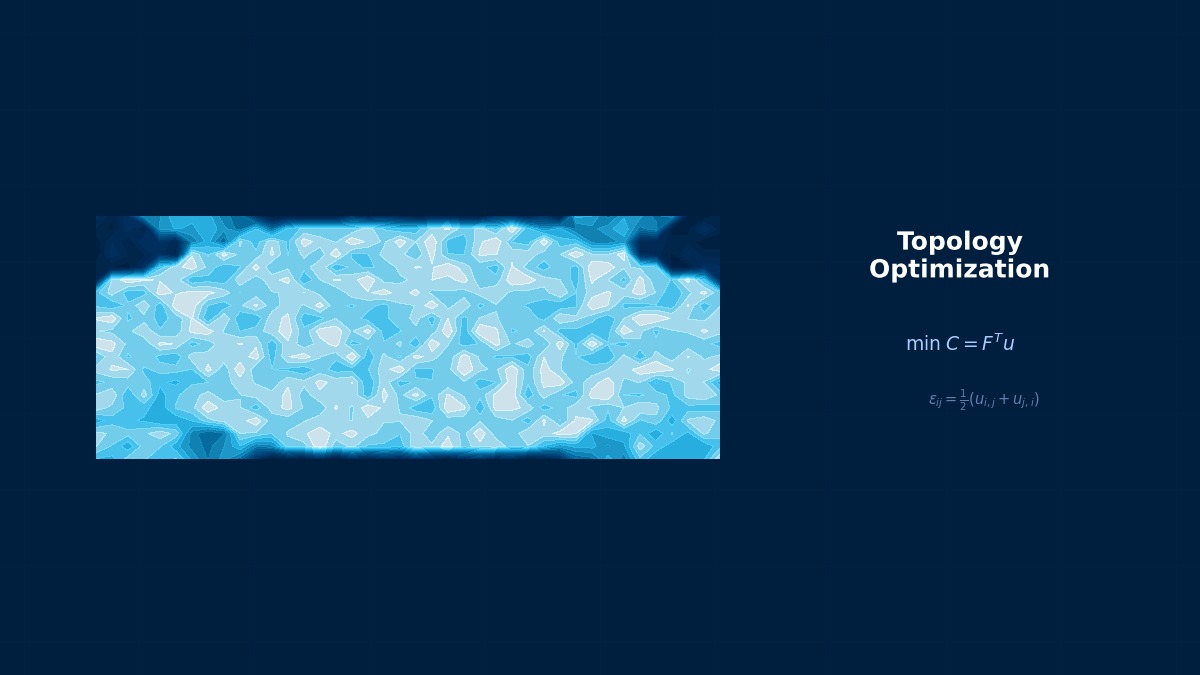
What is the Level Set Method?

🧑‍🎓

Professor, how is the Level Set Method different from the SIMP method?


🎓

The SIMP method represents material presence/absence using the density (0~1) of each element. The Level Set Method directly tracks the boundary (shape) using an implicit function $\phi(\mathbf{x})$. $\phi > 0$: material present, $\phi < 0$: void, $\phi = 0$: boundary.


🧑‍🎓

So the boundary is sharper than with SIMP?


🎓

Yes. SIMP has the problem of gray elements (intermediate density), but Level Set has a consistently clear boundary. However, it is not good at hole nucleation (creating new holes).


Summary

🎓
  • Tracks boundary with implicit function $\phi$ — Avoids SIMP's gray element problem
  • Sharp boundary — Easy CAD conversion
  • Poor at hole nucleation — Depends on initial shape
  • Abaqus TOSCA Level Set — Commercial implementation

  • Coffee Break Yomoyama Talk

    The Level Set Method was invented by Osher and Sethian (1988)

    The Level Set Method is an "interface tracking method" published by Stanley Osher and James Sethian (UC Berkeley) in the Journal of Computational Physics in 1988. Originally developed as a numerical simulation method for flame propagation and water surface waves, its application expanded rapidly to computer vision, medical image processing, and topology optimization through Sethian's works in the 2000s. The application of Level Set to structural optimization was independently published by Wang et al. (2003) and Allaire et al. (2004), and its characteristic is the natural acquisition of smooth boundaries compared to the SIMP method.

    Physical Meaning of Each Term
    • Inertia Term (Mass Term): $\rho \ddot{u}$, meaning "mass × acceleration". Have you ever experienced being thrown forward when slamming on the brakes? That "feeling of being carried forward" is precisely the inertial force. Heavier objects are harder to set in motion and harder to stop once moving. Buildings shake during earthquakes because the ground moves suddenly while the building's mass "gets left behind". In static analysis, this term is set to zero, based on the assumption that "acceleration can be ignored because forces are applied slowly". It absolutely cannot be omitted for impact loads or vibration problems.
    • Stiffness Term (Elastic Restoring Force): $Ku$ or $\nabla \cdot \sigma$. When you stretch a spring, you feel a "force trying to return it", right? That is Hooke's law $F=kx$, which is the essence of the stiffness term. Now a question — an iron rod and a rubber band, which stretches more when pulled with the same force? Obviously the rubber. This "resistance to stretching" is the Young's modulus $E$, which determines stiffness. A common misconception: "high stiffness = strong" is incorrect. Stiffness is "resistance to deformation", strength is "resistance to failure" — they are different concepts.
    • External Force Term (Load Term): Body force $f_b$ (gravity, etc.) and surface force $f_s$ (pressure, contact force, etc.). Think of it this way — the weight of a truck on a bridge is a "force acting on the entire volume" (body force), while the force of the tires pushing on the road surface is a "force acting only on the surface" (surface force). Wind pressure, water pressure, bolt tightening force... all are external forces. A typical mistake here: getting the load direction wrong. Intending "tension" but it becomes "compression" — it sounds like a joke, but it actually happens when coordinate systems are rotated in 3D space.
    • Damping Term: Rayleigh damping $C\dot{u} = (\alpha M + \beta K)\dot{u}$. Try plucking a guitar string. Does the sound continue forever? No, it gradually fades away. That's because vibration energy is converted to heat by air resistance and internal friction in the string. Car shock absorbers work on the same principle — they intentionally absorb vibration energy to improve ride comfort. What if damping were zero? Buildings would continue shaking forever after an earthquake. Since that doesn't happen in reality, setting appropriate damping is crucial.
    Assumptions and Applicability Limits
    • Continuum assumption: Treats material as a continuous medium, ignoring microscopic heterogeneity.
    • Small deformation assumption (for linear analysis): Deformation is sufficiently small compared to initial dimensions, and the stress-strain relationship is linear.
    • Isotropic material (unless otherwise specified): Material properties are independent of direction (anisotropic materials require separate tensor definitions).
    • Quasi-static assumption (for static analysis): Ignores inertial and damping forces, considering only the balance between external and internal forces.
    • Non-applicable cases: For large deformation/large rotation problems, geometric nonlinearity is required. For nonlinear material behavior like plasticity or creep, constitutive law extensions are needed.
    Dimensional Analysis and Unit Systems
    VariableSI UnitNotes / Conversion Memo
    Displacement $u$m (meter)When inputting in mm, unify loads and elastic modulus to MPa/N system.
    Stress $\sigma$Pa (Pascal) = N/m²MPa = 10⁶ Pa. Be careful of unit system inconsistency when comparing with yield stress.
    Strain $\varepsilon$Dimensionless (m/m)Note the distinction between engineering strain and logarithmic strain (for large deformation).
    Elastic modulus $E$PaSteel: ~210 GPa, Aluminum: ~70 GPa. Note temperature dependence.
    Density $\rho$kg/m³In mm system: tonne/mm³ (= 10⁻⁹ tonne/mm³ for steel).
    Force $F$N (Newton)Unify to N in mm system, N in m system.

    Numerical Methods and Implementation

    FEM for Level Set Method

    🎓

    Abaqus TOSCA:

    *TOPOLOGY OPTIMIZATION, LEVELSET for setting. Updates boundary using Hamilton-Jacobi equation.


    Summary

    🎓
    • Abaqus TOSCA Level Set — Commercial implementation
    • Hamilton-Jacobi equation for boundary — Optimizes boundary through time evolution

    • Coffee Break Yomoyama Talk

      Hamilton-Jacobi Equation Drives the Level Set Interface

      In Level Set Method topology optimization, the material/void interface is tracked as the zero level set surface, and the interface evolves over time using the Hamilton-Jacobi equation (∂φ/∂t + v|∇φ|=0). By substituting the shape sensitivity (shape gradient) into the velocity field v, the interface automatically moves in the direction that improves the objective function. NaN propagation and "interface inversion" bugs due to sign errors in the velocity field are the most frequently encountered problems during implementation, and periodic reinitialization of the signed distance function is key to stabilization.

      Linear Elements (1st-order Elements)

      Linear interpolation between nodes. Low computational cost but low stress accuracy. Beware of shear locking (mitigated by reduced integration or B-bar method).

      Quadratic Elements (with Mid-side Nodes)

      Can represent curved deformation. Stress accuracy improves significantly, but degrees of freedom increase by about 2~3 times. Recommended: when stress evaluation is important.

      Full Integration vs Reduced Integration

      Full Integration: Risk of over-constraint (locking). Reduced Integration: Risk of hourglass mode (zero-energy mode). Choose appropriately for the situation.

      Adaptive Mesh

      Automatic refinement based on error indicators (e.g., ZZ estimator). Efficiently improves accuracy in stress concentration areas. Includes h-method (element subdivision) and p-method (order increase).

      Newton-Raphson Method

      Standard method for nonlinear analysis. Updates tangent stiffness matrix every iteration. Achieves quadratic convergence within convergence radius, but computational cost is high.

      Modified Newton-Raphson Method

      Updates tangent stiffness matrix using initial value or every few iterations. Cost per iteration is low, but convergence speed is linear.

      Convergence Criteria

      Force residual norm: $||R|| / ||F_{ext}|| < \epsilon$ (typically $\epsilon = 10^{-3}$ to $10^{-6}$). Displacement increment norm: $||\Delta u|| / ||u|| < \epsilon$. Energy norm: $\Delta u \cdot R < \epsilon$

      Load Increment Method

      Applies total load incrementally in small steps rather than all at once. The arc-length method (Riks method) can track beyond extremum points on the load-displacement curve.

      Analogy: Direct Method vs Iterative Method

      The direct method is like "solving simultaneous equations accurately with pen and paper" — reliable but takes too long for large-scale problems. The iterative method is like "repeatedly guessing to approach the correct answer" — starts with a rough answer but improves accuracy with each iteration. It's the same principle as looking up a word in a dictionary: it's more efficient to estimate where to open it and adjust forward/backward (iterative method) than to search sequentially from the first page (direct method).

      Relationship Between Mesh Order and Accuracy

      1st-order elements are like "approximating a curve with a ruler" — represented by straight line segments, so accuracy is limited. 2nd-order elements are like a "flexible curve" — can represent curved changes, dramatically improving accuracy even with the same mesh density. However, computational cost per element increases, so judgment should be based on total cost-effectiveness.

      Practical Guide

      Level Set in Practice

      🎓

      Because boundaries are sharp and CAD conversion is easy, it is suitable for optimization of 3D printing and precision mechanical parts.


      Practical Checklist

      🎓
      • [ ] Does the initial design contain holes? (Level Set is poor at hole nucleation)
      • [ ] Is convergence confirmed? (May require more iterations than SIMP)

      • Coffee Break Yomoyama Talk

        Apparel Furniture Kartell's Level Set Optimized Chair

        The Italian high-end plastic furniture brand Kartell adopted Level Set topology optimization for the new chair in its "Masters" series announced in 2019. Level Set optimization was performed using Altair Inspire (formerly solidThinking Inspire) for ergonomic load cases (100kg seated weight + lateral impact), optimizing the wall thickness distribution of the polycarbonate chair to reduce component weight from 290g to 210g while maintaining the same strength. The "organically flowing shape" was also adopted as a product design feature and became a topic at the Milano Design Week.

        Analogy: Analysis Flow

        The analysis flow is actually very similar to cooking. First, you buy ingredients (prepare CAD model), do the prep work (mesh generation), apply heat (solver execution), and finally plate it (visualization in post-processing). Here's an important question — which step in cooking is most prone to failure? Actually, it's the "prep work". If mesh quality is poor, the results will be a mess no matter how excellent the solver is.

        Pitfalls Beginners Often Fall Into

        Are you checking mesh convergence? Do you think "the calculation ran = the result is correct"? This is actually the most common trap for CAE beginners. The solver will always return "some answer" for the given mesh. But if the mesh is too coarse, that answer will be far from reality. Confirm that results stabilize with at least three levels of mesh density — neglecting this leads to the dangerous assumption that "the computer gave the answer, so it must be correct".

        Thinking About Boundary Conditions

        Setting boundary conditions is the same as "writing the problem statement" for an exam. If the problem statement is wrong? No matter how accurately you calculate, the answer will be wrong. "Is this surface really fully fixed?" "Is this load really uniformly distributed?" — Correctly modeling real-world constraint conditions is actually the most important step in the entire analysis.

        Software Comparison

        Tools

        🎓
        • Abaqus TOSCA — Level Set support
        • OptiStruct — SIMP method is main
        • Research codes — Implemented at various universities

        • Coffee Break Yomoyama Talk

          Comparison of Level Set Optimization Implementations by Companies

          Commercial implementations of Level Set Method topology optimization followed with Altair OptiStruct (2012~), COMSOL Multiphysics 5.4 (2018~), and Simulia Tosca (2020~). OptiStruct's AMOS (Adaptive Morphology Optimization Strategy), which can automatically apply manufacturing constraints (minimum wall thickness, draft angle), was valued in the automotive industry and adopted for lightweight design of Toyota's knuckle arm.

          The Three Most Important Questions for Selection

          • "What to solve?": Does it support the physical models and element types required for Level Set Method topology optimization? For example, presence of LES support for fluids, and contact/large deformation capabilities for structures make a difference.
          • "Who will use it?": For beginner teams, tools with rich GUI are suitable; for experienced users, flexible script-driven tools are better. Similar to the difference between automatic transmission (GUI) and manual transmission (script) in cars.
          • "How far to expand?": Selection considering future analysis scale expansion (HPC support), deployment to other departments, and integration with other tools leads to long-term cost reduction.

          Advanced Technology

          Advanced Level Set

          🎓
          • Hole nucleation — Automatically generates holes using topological derivative
          • SIMP + Level Set hybrid — Rough shape with SIMP → finish with Level Set

          • Coffee Break Yomoyama Talk

            Origin of Level Set Method: 1988 Osher-Sethian Paper

            Level Set Method for topology optimization is based on the interface tracking algorithm published by Stanley Osher and James Sethian in the Journal of Computational Physics in 1988. Unlike the conventional SIMP method, it has clear boundaries and facilitates manufacturability evaluation, leading to its adoption by Altair solidThinking for the design of an Airbus A350 titanium bracket (42% weight reduction from 1.2kg to 0.7kg).

            Troubleshooting

            Level Set Troubles

            🎓
            • Holes not increasing → Include holes in initial design or use topological derivative for nucleation
            • Slow convergence → Adjust step size

            • Coffee Break Yomoyama Talk

              Countermeasures for Numerical Instability in Level Set Method

              In Level Set Method topology optimization, "boundary disappearance due to numerical diffusion of the Hamilton-Jacobi equation" is a representative convergence failure pattern. COMSOL 6.0 implemented adaptive reinitialization that automatically sets the reinitialization period every 5 optimization iterations, reportedly reducing convergence failure rate for fan blade topology optimization in a Windchill-linked design case from 35% to 8%.

              関連シミュレーター

              この分野のインタラクティブシミュレーターで理論を体感しよう

              シミュレーター一覧

              関連する分野

              熱解析製造プロセス解析V&V・品質保証
              この記事の評価
              ご回答ありがとうございます!
              参考に
              なった
              もっと
              詳しく
              誤りを
              報告
              参考になった
              0
              もっと詳しく
              0
              誤りを報告
              0
              Written by NovaSolver Contributors
              Anonymous Engineers & AI — サイトマップ
              About the Authors