Fatigue Life Prediction of Solder Joints
Fatigue Life Prediction of Solder Joints: Theoretical Foundations
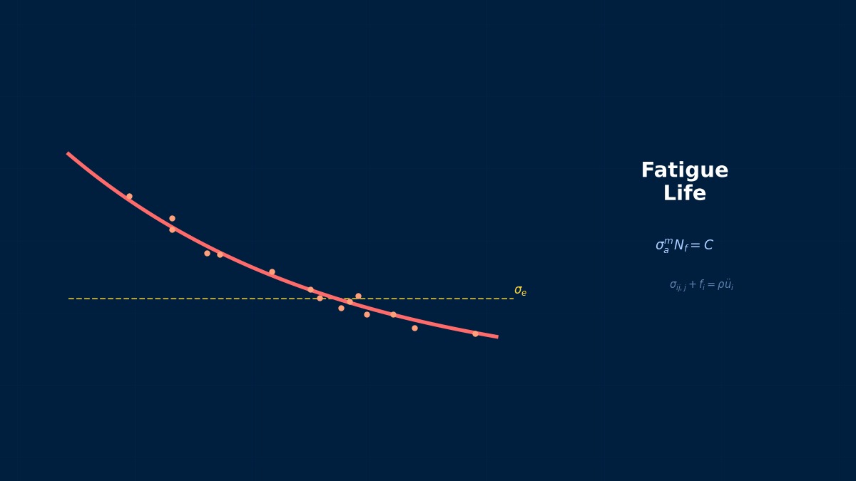
Solder Fatigue
Professor, is solder joint fatigue a reliability issue for electronic devices?
Yes. The difference in CTE (Coefficient of Thermal Expansion) between the PCB and components generates shear strain in the solder with each temperature cycle. This accumulates and leads to fatigue failure. Solder balls in BGAs and QFPs are typical examples.
Coffin-Manson Based Life Prediction
$\Delta\gamma$: Shear strain range. $C_1, C_2$: Solder fatigue constants.
Alternatively, the Darveaux volume-averaged creep energy density method is widely used.
Summary
Creep Fatigue Mechanism of Solder Joints
Solder joints in electronic components (especially BGAs: Ball Grid Arrays) experience repeated deformation due to the thermal expansion difference (CTE difference) between the substrate and component during thermal cycling. The melting point of solder (Sn-3.0Ag-0.5Cu: SAC305 is mainstream) is 217°C, and even at room temperature (25°C), the absolute temperature ratio to the melting point is above 0.6, making creep active. Larger inelastic strain range Δεinelastic per cycle leads to shorter life, and the low-cycle fatigue law (ΔN×Δεinelastic^c=C) independently proposed by Coffin and Manson in 1954 is used as the fundamental theory.
Computational Methods for Fatigue Life Prediction of Solder Joints
Solder Fatigue FEM
1. PCB Assembly FEM Model — PCB (shell or solid) + Components + Solder balls
2. Temperature Cycle — $T_{min}$ → $T_{max}$ (e.g., -40°C → 125°C)
3. Solder Viscoplastic Model — Anand law (integrates creep + plasticity)
4. Extract stabilized cycle strain/energy
5. Calculate life using Coffin-Manson or Darveaux method
Anand Law
Constitutive law for solder (lead-free: SAC305, etc.). Describes temperature-dependent creep + plasticity in a single equation.
Summary
Solder Life Prediction by Darveaux Method
The fatigue life prediction method proposed by Rob Darveaux (Motorola, 1993) consists of three steps: ① Calculation of volume-averaged inelastic strain energy density ΔWAVE of solder balls via FEM, ② Calculation of crack initiation life N0 and crack propagation rate da/dN using experimentally calibrated coefficients K1–K4, and ③ Total life N = N0 + ball diameter / (da/dN). This method is still adopted as the recommended method in ANSIS-STD and JEDEC JEP148 and is widely used for pre-screening before reliability testing.
Fatigue Life Prediction of Solder Joints in Practice
Solder Fatigue Practice
Automotive electronics (-40 to 125°C), Aerospace (-55 to 125°C), Consumer electronics (0 to 60°C).
Practice Checklist
Thermal Cycle Testing of Smartphone Boards
The Apple iPhone 15 Pro's A17 Pro chip (TSMC 3nm) is mounted on the PCB via LGA (Land Grid Array), requiring a minimum of 1000 cycle performance guarantee under −40°C to 125°C thermal cycle testing (JEDEC JESD22-A104 Condition D). Analysis uses an Ansys Sherlock (dedicated electronic reliability tool) PCB assembly model to evaluate CTE mismatch, identifying high-risk solder balls and aiding design changes (judging underfill applicability). Apple regularly validates consistency between physical accelerated testing on actual devices at the Foxconn Zhengzhou factory and analysis.
Fatigue Life Prediction of Solder Joints: Software & Solver Comparison
Solder Fatigue Tools
Electronic Assembly Fatigue Analysis Fatigue Life Prediction of Solder Joints: Software & Solver Comparison
Major tools for electronic solder fatigue analysis: Ansys Sherlock (formerly DfR Solutions Sherlock) integrates board-level fatigue, vibration, and thermal analysis, enabling direct model generation from EDA (Eagle, Altium) data. Simcenter FLOEFD (Siemens) is CFD-focused but can perform ISO 14917-compliant analysis via thermal-structural coupling. Abaqus + Darveaux User Subroutine is widely used for high-precision analysis in research institutions. ProbleSt is relatively low-cost for small/medium electronic manufacturers. Shellex has strong integration with board-specific CAD and is adopted by Japanese companies like Denso and Panasonic.
Advanced Technologies
Solder Fatigue Advanced
Improving Accuracy of Strain Energy Density Method
The accuracy of the Darveaux method strongly depends on model mesh density and solder viscoelastic constitutive law. The Anand viscoplastic model (proposed in 1985 by MIT Professor Lallit Anand) describes solder's temperature- and strain rate-dependent plasticity with one set of 9 constants; constants for SAC305 were experimentally identified by Pang et al. (2008, Nanyang Technological University). However, for modeling acceleration factors in AGT (Accelerated Global Thermal) testing, extrapolating the Anand model's creep behavior to real environments is effective when combined with a CoffinMansonArrhenius composite model based on data at 25–50°C.
Fatigue Life Prediction of Solder Joints: Common Issues & Debugging
Solder Fatigue Troubles
Related Topics
Experience the theory firsthand with the interactive simulator for this field
All Simulators