1次元定常熱伝導

Category: 熱解析 | Integrated 2026-04-06
CAE visualization for conduction 1d theory - technical simulation diagram
1次元定常熱伝導

Theory and Physics

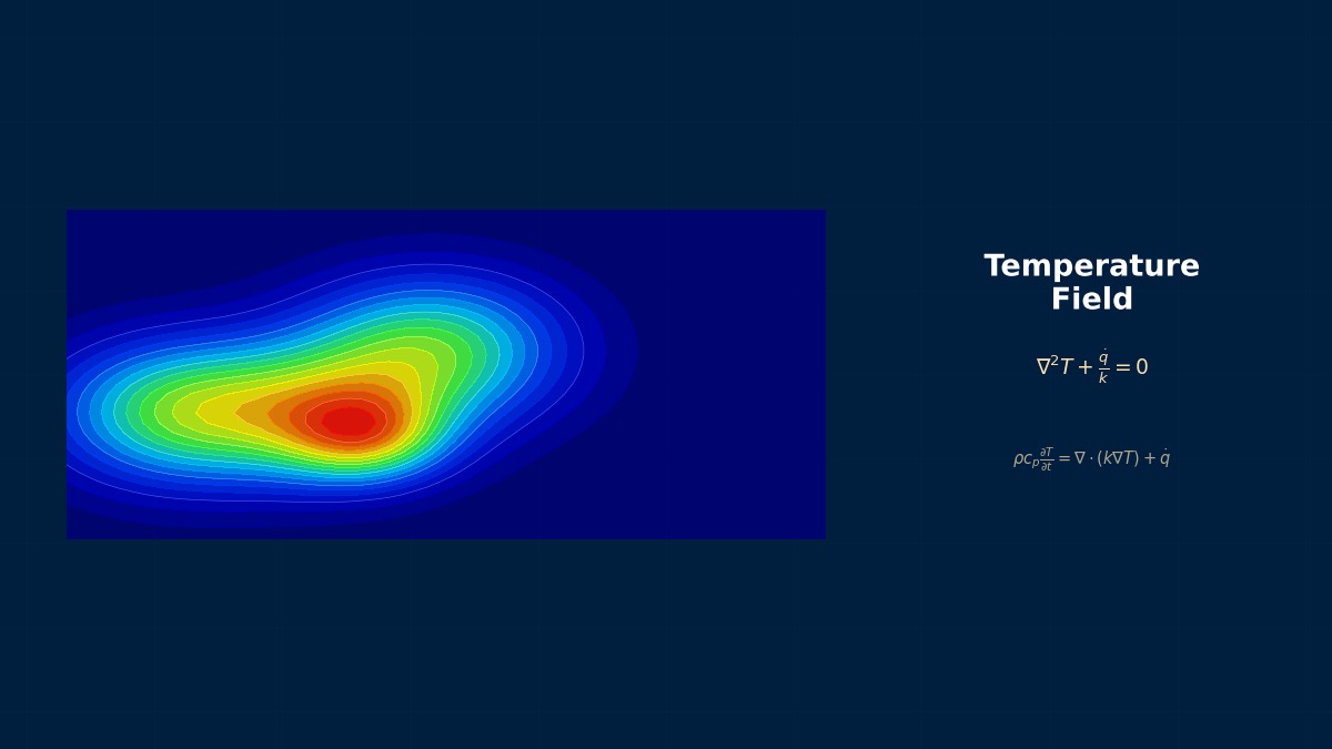
Fundamentals of 1D Steady-State Heat Conduction

🧑‍🎓

Professor, in what actual situations is 1D steady-state heat conduction used?


🎓

It is applied to problems where a temperature gradient exists in only one direction, such as in flat plates, cylinders, and spherical shells. Typical examples include thermal insulation evaluation of walls, design of pipe insulation, and calculation of allowable current for electrical wires.


Governing Equation

🎓

The governing equation for 1D steady-state with internal heat generation is as follows.


$$\frac{d}{dx}\left(k \frac{dT}{dx}\right) + \dot{q}_v = 0$$

If $k$ is constant and there is no heat generation, it becomes $\frac{d^2T}{dx^2} = 0$, and the temperature distribution becomes linear.


🧑‍🎓

What happens when there is uniform heat generation?


🎓

For fixed surface temperatures $T(0)=T_1$, $T(L)=T_2$ and uniform $\dot{q}_v$,


$$T(x) = T_1 + (T_2 - T_1)\frac{x}{L} + \frac{\dot{q}_v}{2k}x(L-x)$$

A quadratic curve is superimposed. The maximum temperature is not necessarily at the center; it becomes biased when $T_1 \neq T_2$.


Concept of Thermal Resistance

🎓

The electrical circuit analogy is very effective for 1D heat conduction. The thermal resistance for a flat plate is


$$R_{cond} = \frac{L}{kA}$$

The convective thermal resistance is $R_{conv} = \frac{1}{hA}$. These are connected in series or parallel to estimate the overall temperature drop.


🧑‍🎓

It's exactly like Ohm's law. $\Delta T = qR$ corresponds to V=IR.


🎓

Exactly. This concept of thermal resistance networks also forms the basis for FloTHERM's Compact Thermal Model and JEDEC's DELPHI model.

Coffee Break Trivia

Fourier's Heat Equation, Conceived in Prison

Joseph Fourier (1768–1830) continued his research even during his imprisonment after returning from the Egyptian expedition in 1798. He completed the 1D heat conduction equation in his 1822 publication 'Analytical Theory of Heat', but the Royal Academy rejected the initial manuscript (1807) for 12 years, citing "lack of rigor".

Physical Meaning of Each Term
  • Heat Storage Term $\rho c_p \partial T/\partial t$: Rate of thermal energy storage per unit volume. 【Everyday Example】 An iron frying pan heats up slowly and cools down slowly, while an aluminum pot heats up quickly and cools down quickly—this is due to the difference in the product of density $\rho$ and specific heat $c_p$ (Heat Capacity). Objects with large heat capacity experience slower temperature changes. Water has a very high specific heat (4,186 J/(kg·K)), which is why temperatures near the sea are more stable than inland. In transient analysis, this term determines the rate of temperature change over time.
  • Heat Conduction Term $\nabla \cdot (k \nabla T)$: Heat conduction based on Fourier's law. Heat flux proportional to the temperature gradient. 【Everyday Example】 When you put a metal spoon in a hot pot, the handle gets hot—because metal has a high thermal conductivity $k$, heat transfers quickly from the high-temperature side to the low-temperature side. A wooden spoon doesn't get hot because its $k$ is small. Insulation materials (like glass wool) have extremely small $k$, making heat transfer difficult even with a temperature gradient. This is a mathematical formulation of the natural tendency: "Heat flows where there is a temperature difference."
  • Convection Term $\rho c_p \mathbf{u} \cdot \nabla T$: Heat transport accompanying fluid motion. 【Everyday Example】 Feeling cool when a fan blows on you is because the wind (fluid flow) carries away the warm air near your skin and supplies fresh, cool air—this is forced convection. The ceiling area of a room becoming warm with heating is due to natural convection where heated air rises due to buoyancy. The fan in a PC's CPU cooler also dissipates heat via forced convection. Convection is an order of magnitude more efficient at heat transport than conduction.
  • Heat Source Term $Q$: Internal heat generation (Joule heat, chemical reaction heat, radiation absorption, etc.). Unit: W/m³. 【Everyday Example】 A microwave oven heats food via microwave absorption inside the food (volumetric heating). The heater wire in an electric blanket warms up via Joule heating ($Q = I^2 R / V$). Heat generation during charging/discharging of lithium-ion batteries and friction heat from brake pads are also considered as heat sources in analysis. Unlike boundary conditions that supply heat to the "surface" from the outside, the heat source term represents energy generation "inside" the material.
Assumptions and Applicability Limits
  • Fourier's Law: Linear relationship where heat flux is proportional to temperature gradient (non-Fourier heat conduction is needed for extremely low temperatures or ultra-short pulse heating)
  • Isotropic Thermal Conductivity: Thermal conductivity is independent of direction (anisotropy must be considered for composite materials or single crystals)
  • Temperature-Independent Material Properties (Linear Analysis): Assumption that material properties do not depend on temperature (temperature dependence is needed for large temperature differences)
  • Treatment of Thermal Radiation: View factor method for surface-to-surface radiation; DO method or P1 approximation for participating media
  • Non-Applicable Cases: Consideration of latent heat is necessary for phase change (melting/solidification). Thermal-stress coupling is essential for extreme temperature gradients
Dimensional Analysis and Unit Systems
VariableSI UnitNotes / Conversion Memo
Temperature $T$K (Kelvin) or CelsiusBe careful not to confuse absolute temperature and Celsius. Always use absolute temperature for radiation calculations.
Thermal Conductivity $k$W/(m·K)Steel: ~50, Aluminum: ~237, Air: ~0.026
Heat Transfer Coefficient $h$W/(m²·K)Natural Convection: 5–25, Forced Convection: 25–250, Boiling: 2,500–25,000
Specific Heat $c_p$J/(kg·K)Distinguish between specific heat at constant pressure and constant volume (important for gases)
Heat Flux $q$W/m²Neumann condition as a boundary condition

Numerical Methods and Implementation

Discretization by Finite Difference Method

🧑‍🎓

It seems like we could solve 1D problems by hand calculation, but why use numerical methods?


🎓

Analytical solutions cannot be obtained when there is temperature-dependent thermal conductivity $k(T)$ or non-uniform heat generation. Discretizing on a uniform grid using FDM gives:


$$k_{i+1/2}\frac{T_{i+1}-T_i}{\Delta x} - k_{i-1/2}\frac{T_i-T_{i-1}}{\Delta x} + \dot{q}_{v,i}\Delta x = 0$$

Here, $k_{i+1/2}$ is evaluated using the harmonic mean at the cell interface. $k_{i+1/2} = \frac{2k_i k_{i+1}}{k_i + k_{i+1}}$


🧑‍🎓

Why use the harmonic mean?


🎓

To maintain heat flux continuity at interfaces between different materials. Using the arithmetic mean could lead to discontinuous heat flux at the interface. This treatment is also used in CFD solvers.


1D Analysis by FEM

🎓

In 1D FEM, two-node linear elements are used. The element thermal conductivity matrix is:


$$[K^e] = \frac{kA}{L_e}\begin{bmatrix}1 & -1\\-1 & 1\end{bmatrix}$$

It has exactly the same form as a structural spring element. For convective boundaries, add the term $hA\begin{bmatrix}0&0\\0&1\end{bmatrix}$ to the right end.


🧑‍🎓

It seems like we could even implement this in Excel for 1D problems.


🎓

Yes. For educational purposes, implementing about 10 elements in Excel is very effective for understanding the essence of FEM. In practice, of course, we use general-purpose solvers, but having a custom tool for verification can be very useful.

Coffee Break Trivia

The Origin of Finite Difference Method is Richardson

The method by Lewis Fry Richardson (1910), who approximated fluid equations with finite differences, is the prototype for numerical solutions of 1D heat conduction. He is famous for a grand experiment during World War I, using a finite difference grid for manual weather forecasting and mobilizing 64 "human computers". He was a pioneer who introduced the concept of computational accuracy to numerical thermodynamics.

Linear Elements vs. Quadratic Elements

In heat conduction analysis, linear elements often provide sufficient accuracy. Quadratic elements are recommended for regions with steep temperature gradients (e.g., thermal shock).

Heat Flux Evaluation

Calculated from the temperature gradient within an element. Smoothing may be required, similar to nodal stresses.

Convection-Diffusion Problem

When the Peclet number is high (convection-dominated), upwinding stabilization (e.g., SUPG) is needed. Not required for pure heat conduction problems.

Time Step for Transient Analysis

Set a time step sufficiently smaller than the characteristic thermal diffusion time $\tau = L^2 / \alpha$ ($\alpha$: Thermal Diffusivity). Automatic time step control is effective for rapid temperature changes.

Nonlinear Convergence

Nonlinearity due to temperature-dependent material properties is often mild, and Picard iteration (direct substitution method) is often sufficient. Newton's method is recommended for strong nonlinearities like radiation.

Steady-State Analysis Convergence Criterion

Convergence is judged when the temperature change at all nodes falls below a threshold (e.g., $|\Delta T| / T_{max} < 10^{-5}$).

Analogy for Explicit and Implicit Methods

The explicit method is like "weather forecasting that predicts the next step using only current information"—fast to compute but unstable with large time steps (misses storms). The implicit method is like "prediction that also considers future states"—stable even with large time steps but requires solving equations at each step. For problems without rapid temperature changes, using the implicit method with larger time steps is more efficient.

Practical Guide

Utilization in Design Calculations

🧑‍🎓

Are 1D models really used in actual work? Even though we have 3D.


🎓

1D models are overwhelmingly efficient in the conceptual design stage. Determining insulation thickness for walls, selecting pipe insulation, and sizing electrical wires can be done with sufficient accuracy using 1D calculations.


Practical Example: Pipe Insulation Design

🎓

For a steam pipe with an outer diameter of 50mm (150°C) wrapped with glass wool insulation ($k=0.04$ W/(m K)), with ambient air at 25°C and an external surface heat transfer coefficient $h=10$ W/(m²K):


$$q = \frac{2\pi L(T_i - T_\infty)}{\frac{\ln(r_o/r_i)}{k_{ins}} + \frac{1}{h r_o}}$$

With an insulation thickness of 50mm, $r_i=25$mm, $r_o=75$mm, the heat loss per unit length is approximately 20 W/m.


🧑‍🎓

This can be calculated by hand in about 10 seconds. No need to run a 3D simulation.


🎓

Exactly. However, pipe elbows, branches, and flange sections exhibit 2D/3D effects, so we use 1D for overall heat loss calculation and 3D for local temperature evaluation.


Result Verification

🎓

Using 1D theoretical solutions to verify 3D analysis results is very effective.


Verification Item1D Theoretical Value3D Analysis ValueAcceptance Criterion
Maximum TemperatureCalculated from theoretical formulaSolver outputDifference within 5%
Heat Flow Rate$q=kA\Delta T/L$Surface integralDifference within 2%
Temperature Gradient$dT/dx = -q/(kA)$Path plotDistribution matches
🧑‍🎓

So if you understand 1D, you can quickly verify 3D results.


🎓

Just checking "if the order of magnitude is correct" can prevent 80% of design errors. That is the greatest value of 1D models.

Coffee Break Trivia

The Golden Rule of Furnace Wall Design

Blast furnace walls in steelmaking are often designed using 1D steady-state approximations. Nippon Steel & Sumitomo Metal (now Nippon Steel) uses a three-layer structure of refractory brick → insulating castable → steel plate, optimizing λ and thickness to maintain 1600°C on the inside and 60°C on the outside. Reducing heat loss per unit area of the furnace wall directly impacts annual energy costs.

Analogy for Analysis Flow

Think of the thermal analysis flow as "designing a bath reheating system". Decide the bathtub shape (analysis target), set the initial water temperature (initial condition) and outside air temperature (boundary condition), and adjust the reheater output (heat source). Predicting "whether it will become lukewarm after 2 hours?" by calculation—this is the essence of transient thermal analysis.

Common Pitfalls for Beginners

"Can I ignore radiation?" — Usually OK around room temperature. But it's a different story above several hundred degrees. Radiative heat transfer is proportional to the fourth power of temperature, so it overwhelms convection at high temperatures. Have you ever experienced how different the perceived temperature is in the sun versus in the shade on a sunny day? That's the power of radiation. Ignoring radiation in the analysis of industrial furnaces or engine components is like insisting "sunlight doesn't matter" on a scorching hot day.

Thinking About Boundary Conditions

Think of the heat transfer coefficient $h$ as "the insulation performance of a window". Large $h$ = thin window = heat escapes easily. Small $h$ = double-glazed window = heat escapes slowly. This single value can greatly change the results, so referencing literature values or identification through experiments is important. Are you just putting in "let's say 10 W/(m²·K)..." arbitrarily?

Software Comparison

Handling by Tool

🧑‍🎓

Please tell me how to handle 1D heat conduction in each software.


🎓

Let's compare implementation methods in general-purpose FEM solvers.


ToolElement TypeKey Setup Points
ANSYS MechanicalLINK33 (Thermal Conduction Bar)Define real constant for cross-sectional area. For convection, use SURF151/SURF152.
関連シミュレーター

この分野のインタラクティブシミュレーターで理論を体感しよう

シミュレーター一覧

関連する分野

構造解析流体解析製造プロセス解析
この記事の評価
ご回答ありがとうございます!
参考に
なった
もっと
詳しく
誤りを
報告
参考になった
0
もっと詳しく
0
誤りを報告
0
Written by NovaSolver Contributors
Anonymous Engineers & AI — サイトマップ
About the Authors
Sponsored by ○○株式会社