3D Steady-State Heat Conduction
3D Steady-State Heat Conduction: Theoretical Foundations
Fundamentals of 3D Steady-State Heat Conduction
What changes when moving from 2D to 3D heat conduction analysis?
Since the temperature field changes in three directions, it targets problems where shape simplification is not effective. Many real-world problems like engine blocks, molds, and electronic enclosures are inherently three-dimensional.
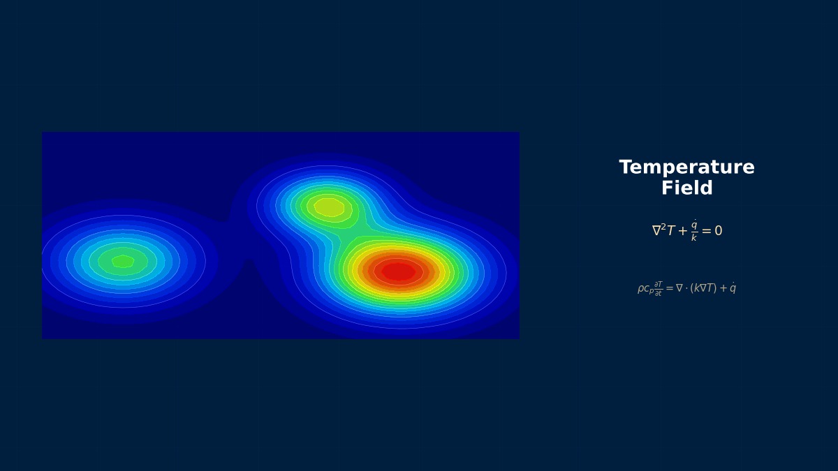
Governing Equation
The 3D steady-state heat conduction equation is
Expanding it gives
For anisotropic materials, $k_x \neq k_y \neq k_z$.
There are almost no analytical solutions in 3D, right?
For a rectangular prism with simple boundary conditions on each face, a triple series solution exists, but in practice, numerical methods are essential. Discretization using FEM solid elements (tetrahedra, hexahedra) is the standard approach.
Types of Boundary Conditions
In 3D problems, different boundary conditions can be set for each face.
| Face | Condition | Example |
|---|---|---|
| Heat Generation Surface | Heat Flux q [W/m2] | IC Heat Generation Surface |
| Heat Dissipation Surface | Convection h, T∞ | Heat Sink Outer Surface |
| Contact Surface | Contact Conductance | Bolted Joint |
| Symmetry Plane | Adiabatic (q=0) | Utilizing Symmetry |
| Fixed Temperature | T = const | Cooling Water Surface |
Being able to change conditions per face is a strength of 3D, isn't it?
Correct. In 1D, you can only treat the whole system uniformly, but in 3D, you can set individual conditions for each face and region, allowing you to create models faithful to real-world physics.
General Form of the 3D Heat Conduction Equation
The 3D steady-state heat conduction equation ∇·(λ∇T)+q̇=0 reduces to Laplace's equation if λ is isotropic and homogeneous and there is no internal heat generation. The "Green's function" introduced by Green (1828) became the foundation for solving the 3D Poisson equation and was later applied to the Helmholtz equation and electromagnetism. Green is also known for his origins as the self-taught son of a baker.
Computational Methods for 3D Steady-State Heat Conduction
FEM Element Selection
Which elements should I use for 3D thermal analysis?
Comparison of 3D heat conduction elements.
| Element Type | Number of Nodes | Temperature Distribution | Accuracy | Mesh Generation |
|---|---|---|---|---|
| 4-Node Tetrahedron (TET4) | 4 | Linear | Low | Easy automatic meshing |
| 10-Node Tetrahedron (TET10) | 10 | Quadratic | High | Easy automatic meshing |
| 8-Node Hexahedron (HEX8) | 8 | Trilinear | Medium–High | Requires structured mesh |
| 20-Node Hexahedron (HEX20) | 20 | Quadratic | Very High | Difficult to generate |
In Ansys, SOLID70(HEX8), SOLID87(TET10), SOLID90(HEX20) are representative thermal elements. In Abaqus, they correspond to DC3D4, DC3D10, DC3D8, DC3D20.
Is TET10 a safe choice in practice?
Considering compatibility with automatic meshing, TET10 has high versatility. However, if the shape allows hexahedral meshing, HEX8 can reduce the number of elements. Using Ansys Meshing's Multizone or Sweep methods allows priority generation of HEX elements.
Handling Large-Scale Problems
Element count increases rapidly in 3D problems. Countermeasures for cases exceeding 1 million elements:
- Iterative Solver: PCG method + AMG preconditioner uses about 1/10 the memory of direct methods
- Parallel Computing: Utilize multiple cores with Ansys DMP (Distributed Memory Parallel)
- Submodeling: Refine a local model using the temperature field from the global model as boundary conditions
How do you do submodeling specifically?
Obtain a steady-state solution with a coarse global model, transfer the temperature to the boundary faces of the region of interest, and solve a refined model. This can be easily set up with the Submodel command in Ansys Workbench. Even using a mesh 10 times finer for 10% of the total area results in computational cost roughly 1/100th of refining the entire model.
Birth of FEM Tetrahedral Elements
The tetrahedral element, essential for 3D thermal analysis, was proposed in 1960 by Turner et al. in NASA-sponsored research. Initially for structural analysis, its adaptation to thermal analysis was systematized by Wilson and Bathe in the 1970s. The origins of C3D10 (10-node quadratic tetrahedron) used in current Abaqus/Standard and Ansys Mechanical also date back to this era.
3D Steady-State Heat Conduction in Practice
Guidelines for Shape Simplification
If you use CAD data as-is, the element count explodes, right?
CAD geometry cleanup determines the success or failure of 3D thermal analysis.
| Simplification Item | Effect | Caution |
|---|---|---|
| Removing Small Fillets | 50% reduction in element count | Guideline: below 0.5mm |
| Shelling Thin-Walled Parts | No elements needed in thickness direction | Not possible if gradients in thickness direction are important |
| Omitting Bolt Holes | Avoids local refinement | Limited to those not affecting heat paths |
| Utilizing Symmetry | 1/2 to 1/8 model | Boundary conditions must also be symmetric |
So you simplify in SpaceClaim (Ansys) or Design Modeler, right?
Correct. Ansys Discovery Live allows you to see the temperature field in real-time while modifying the geometry, enabling quick judgment of which geometric features affect the temperature field.
Mesh Strategy
Mesh guidelines for 3D steady-state heat conduction:
- Near heat sources: Minimum element size = 1/5 or less of the heat source size
- Far field: Can be coarse (temperature gradient is small)
- Material interfaces: Mesh aligned with the interface (shared nodes or Tied Contact)
- Thin-walled parts: At least 3 layers in the thickness direction
What criteria do you use for convergence verification?
If the maximum temperature is the quantity of interest, it's sufficient if the change in maximum temperature is within 1% when the mesh is refined by a factor of 2. However, local heat flux converges slower, so verification with three or more mesh refinement levels is advised.
Thermal Analysis of an Automotive Engine Head
Toyota used 3D steady-state thermal analysis in developing the GR Yaris (2020) to optimize the temperature distribution around the combustion chamber of the aluminum cast head. They reduced the maximum temperature near the fuel injection nozzle by about 25°C compared to previous designs, achieving both knock resistance and thermal efficiency. The analysis model had over 2 million nodes, with a computation time of about 4 hours on an 8-core PC.
Experience the theory firsthand with the interactive simulator for this field
All Simulators