2次元定常熱伝導

Category: 熱解析 | Integrated 2026-04-06
CAE visualization for conduction 2d theory - technical simulation diagram
2次元定常熱伝導

Theory and Physics

Fundamentals of 2D Heat Conduction

🧑‍🎓

How is 2D steady-state heat conduction extended from 1D?


🎓

It's a problem where temperature changes in two directions. Representative examples include in-plane temperature distribution on circuit boards, cross-sectional temperature fields in molds, and thermal bridge evaluation in building walls.
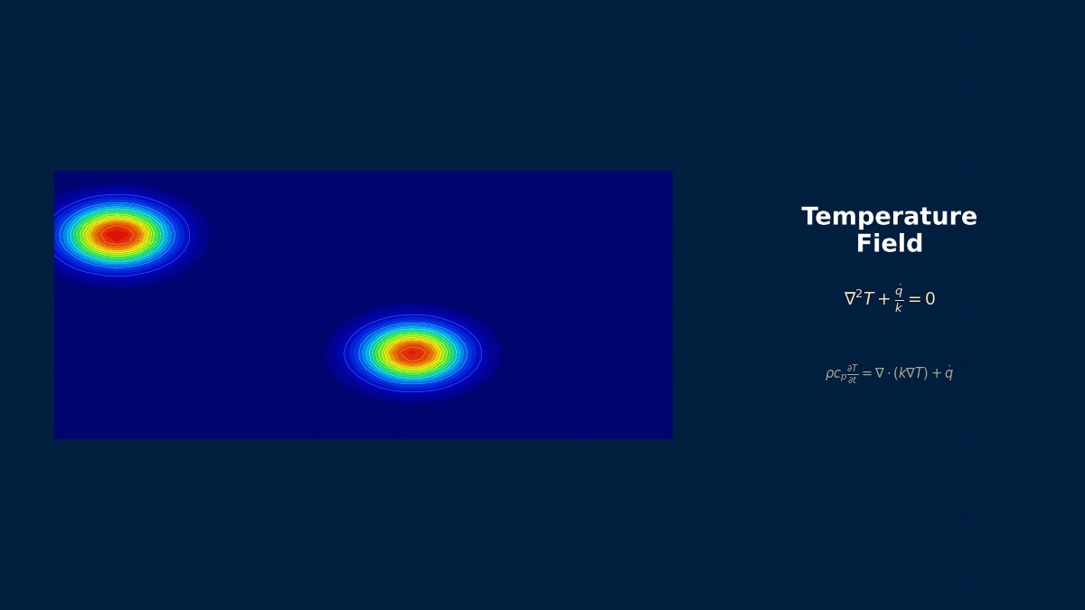

Governing Equation

🎓

The 2D steady-state heat conduction equation for isotropic materials is as follows.


$$\frac{\partial}{\partial x}\left(k\frac{\partial T}{\partial x}\right) + \frac{\partial}{\partial y}\left(k\frac{\partial T}{\partial y}\right) + \dot{q}_v = 0$$

If $k$ is constant and there is no heat generation, it reduces to the Laplace equation $\nabla^2 T = 0$.


🧑‍🎓

Are there analytical solutions?


🎓

For a rectangular domain with specified temperatures on each side, a series solution can be obtained using the separation of variables method. For example, for a square domain where three sides are 0°C and one side is $T_0$:


$$T(x,y) = \sum_{n=1,3,5,...}^{\infty} \frac{4T_0}{n\pi} \frac{\sinh(n\pi y/L)}{\sinh(n\pi)} \sin\frac{n\pi x}{L}$$

This solution is extremely important as a verification benchmark for FEM codes.


Shape Factor Method

🎓

As a convenient method to treat 2D geometric effects in a 1D manner, there is the shape factor $S$.


$$q = kS\Delta T$$

For example, the heat loss from a buried pipe in the ground can be evaluated with $S = 2\pi L / \cosh^{-1}(D/r)$. Textbooks (Incropera et al.) summarize $S$ for major shapes.


🧑‍🎓

So, using the shape factor, 2D problems can be solved by hand calculation.


🎓

That's right. However, for complex shapes, the shape factor is unknown, so we solve them using FEM. In practice, it's common to back-calculate the shape factor value from FEM results and reuse it for similar designs.

Coffee Break Trivia

Laplace Equation and the Beauty of Analytical Solutions

2D steady-state heat conduction is described by ∇²T=0 (Laplace equation). The analytical solution for a rectangular plate shown by Fourier in 1822 is expressed as a sine series and is still used today as a verification benchmark. The Laplace equation has the same form as electric potential and velocity potential, and 19th-century physicists praised this unity as "the deep beauty of nature."

Physical Meaning of Each Term
  • Heat Storage Term $\rho c_p \partial T/\partial t$: Rate of thermal energy storage per unit volume. 【Everyday Example】 An iron frying pan is slow to heat up and cool down, while an aluminum pot heats up and cools down quickly—this is due to the difference in the product of density $\rho$ and specific heat $c_p$ (Heat Capacity). Objects with large heat capacity have slower temperature changes. Water has a very large specific heat (4,186 J/(kg·K)), so temperatures near the sea are more stable than inland. In transient analysis, this term determines the rate of temperature change over time.
  • Heat Conduction Term $\nabla \cdot (k \nabla T)$: Heat conduction based on Fourier's law. Heat flux proportional to the temperature gradient. 【Everyday Example】 When you put a metal spoon in a hot pot, the handle gets hot—because metal has a high thermal conductivity $k$, heat quickly transfers from the high-temperature side to the low-temperature side. A wooden spoon doesn't get hot because its $k$ is small. Insulation materials (e.g., glass wool) have extremely small $k$, so heat hardly transfers even with a temperature gradient. This is a mathematical formulation of the natural tendency that "heat flows where there is a temperature difference."
  • Convection Term $\rho c_p \mathbf{u} \cdot \nabla T$: Heat transport accompanying fluid motion. 【Everyday Example】 Feeling cool when a fan blows on you is because the wind (fluid flow) carries away the warm air near your skin and supplies fresh, cold air—this is forced convection. The ceiling area of a room getting warm with heating is due to natural convection where heated air rises due to buoyancy. The fan in a PC's CPU cooler also dissipates heat via forced convection. Convection is an order of magnitude more efficient heat transport method than conduction.
  • Heat Source Term $Q$: Internal heat generation (Joule heat, chemical reaction heat, radiation absorption, etc.). Unit: W/m³. 【Everyday Example】 A microwave oven heats food via microwave absorption inside the food (volumetric heating). The heater wire in an electric blanket warms up via Joule heating ($Q = I^2 R / V$). Heat generation during charging/discharging of lithium-ion batteries and friction heat from brake pads are also considered as heat sources in analysis. Unlike boundary conditions that supply heat from the "surface" externally, the heat source term represents energy generation "inside" the material.
Assumptions and Applicability Limits
  • Fourier's Law: Linear relationship where heat flux is proportional to temperature gradient (non-Fourier heat conduction is needed for extremely low temperatures or ultra-short pulse heating)
  • Isotropic Thermal Conductivity: Thermal conductivity does not depend on direction (anisotropy must be considered for composite materials, single crystals, etc.)
  • Temperature-Independent Material Properties (Linear Analysis): Assumption that material properties do not depend on temperature (temperature dependence is needed for large temperature differences)
  • Treatment of Thermal Radiation: View factor method for surface-to-surface radiation; DO method or P1 approximation for participating media
  • Non-Applicable Cases: Consideration of latent heat is necessary for phase change (melting/solidification). Thermal-stress coupling is essential for extreme temperature gradients
Dimensional Analysis and Unit Systems
VariableSI UnitNotes / Conversion Memo
Temperature $T$K (Kelvin) or CelsiusBe careful not to confuse absolute temperature and Celsius. Always use absolute temperature for radiation calculations.
Thermal Conductivity $k$W/(m·K)Steel: ~50, Aluminum: ~237, Air: ~0.026
Heat Transfer Coefficient $h$W/(m²·K)Natural Convection: 5–25, Forced Convection: 25–250, Boiling: 2,500–25,000
Specific Heat $c_p$J/(kg·K)Distinguish between specific heat at constant pressure and constant volume (important for gases)
Heat Flux $q$W/m²Neumann condition as a boundary condition

Numerical Methods and Implementation

2D Discretization by FEM

🧑‍🎓

What kind of elements are used for 2D problems in FEM?


🎓

For 2D heat conduction, there are triangular and quadrilateral elements.


ElementNumber of NodesTemperature DistributionAccuracy
3-node triangle3LinearLow (constant temperature gradient)
6-node triangle6QuadraticHigh
4-node quadrilateral4BilinearMedium
8-node quadrilateral8QuadraticHigh
🎓

The 3-node triangle has a constant temperature gradient within the element, so accuracy is poor unless refined. In practice, 6-node triangles or 8-node quadrilaterals are recommended.


🧑‍🎓

Which is better, quadrilateral or triangle?


🎓

For the same number of nodes, quadrilaterals have higher accuracy. However, triangles (tetrahedra) are easier to generate for automatic meshing of complex shapes. Choosing hex-dominant meshing in Ansys provides a good balance.


Finite Difference Method (2D)

🎓

Central differencing on a uniform grid is:


$$k\frac{T_{i+1,j} - 2T_{i,j} + T_{i-1,j}}{\Delta x^2} + k\frac{T_{i,j+1} - 2T_{i,j} + T_{i,j-1}}{\Delta y^2} + \dot{q}_v = 0$$

If $\Delta x = \Delta y$, it becomes the famous 5-point stencil. This can be implemented in Excel or custom Python code for verification.


🧑‍🎓

Verifying commercial solver results with custom code is a solid approach.


🎓

Especially for 2D verification, it can be written in a few dozen lines of Excel VBA or Python, so there's no reason not to do it.

Coffee Break Trivia

FDM Central Differencing is 2nd Order Accurate

The central differencing scheme for 2D FDM has second-order spatial accuracy; halving the grid spacing reduces the error to 1/4. In the 1960s, NASA performed 2D thermal analysis of rocket nozzles on an IBM 704, which took several hours even for a 128×128 grid. On a modern PC, the same calculation finishes in less than 0.01 seconds. Computational speed has improved by over 10⁹ times in 50 years.

Linear Elements vs. Quadratic Elements

In heat conduction analysis, linear elements often provide sufficient accuracy. For regions with steep temperature gradients (e.g., thermal shock), quadratic elements are recommended.

Heat Flux Evaluation

Calculated from the temperature gradient within the element. Smoothing may be required, similar to nodal stresses.

Convection-Diffusion Problem

When the Peclet number is high (convection-dominated), upwinding stabilization (SUPG, etc.) is needed. Not required for pure heat conduction problems.

Time Step for Transient Analysis

Set a time step sufficiently smaller than the characteristic thermal diffusion time $\tau = L^2 / \alpha$ ($\alpha$: Thermal Diffusivity). Automatic time step control is effective for rapid temperature changes.

Nonlinear Convergence

Nonlinearity due to temperature-dependent material properties is often mild, and Picard iteration (direct substitution) is often sufficient. Newton's method is recommended for strong nonlinearities like radiation.

Steady-State Analysis Convergence Criterion

Convergence is judged when the temperature change at all nodes falls below a threshold (e.g., $|\Delta T| / T_{max} < 10^{-5}$).

Analogy for Explicit and Implicit Methods

Explicit method is like "predicting the next step using only current information, like a weather forecast"—calculation is fast but unstable with large time steps (misses storms). Implicit method is like "prediction considering future states"—stable even with large time steps, but requires solving equations at each step. For problems without rapid temperature changes, using large time steps with the implicit method is more efficient.

Practical Guide

Scenarios for Utilizing 2D Models

🧑‍🎓

Since 3D analysis is mainstream, what are the advantages of deliberately using a 2D model?


🎓

The computational cost is orders of magnitude smaller. 2D is optimal for parametric studies running dozens of cases or for problems where temperature gradients in the cross-sectional direction are dominant.


Practical Example: Thermal Bridge Analysis of PCB

🎓

When modeling the cross-section of a multilayer PCB, each layer (copper foil, prepreg, core) is arranged as a strip with different $k$. The equivalent thermal conductivity differs greatly between an L1 layer with 80% copper coverage and an L3 layer with 20%.


LayerThickness [um]In-plane k [W/(mK)]Through-plane k [W/(mK)]
L1 (Cu 80%)353181.1
Prepreg1000.30.3
L2 (Cu 50%)351990.55
Core8000.30.3
🧑‍🎓

The difference between in-plane and through-plane is over two orders of magnitude.


🎓

PCB substrates are extremely anisotropic materials. 2D cross-sectional analysis evaluates through-plane temperature gradients and via effects, while in-plane direction is corrected using spreading resistance. This is the technique also used in the internal modeling of FloTHERM and Icepak.


Utilizing Symmetry

🎓

Utilizing symmetry can significantly reduce computational scale.


  • 1-axis symmetry: 1/2 model, adiabatic condition on the symmetry plane
  • 2-axis symmetry: 1/4 model
  • Cyclic symmetry: Model only one repeating unit

🧑‍🎓

Why does the symmetry plane become an adiabatic condition?


🎓

If the temperature field is mirror-symmetric across the symmetry plane, the temperature gradient crossing the plane is zero, meaning the heat flux is zero. It's a natural consequence when you think about it physically.

Coffee Break Trivia

2D Temperature Map of a CPU Die

In 2003, Intel extensively used 2D steady-state thermal analysis for hot spot management in the Pentium 4 "Prescott" core (90 nm process, TDP 84 W). The maximum temperature difference on the die exceeded 20°C, and locations of current density concentration were identified using 2D maps to redesign the wiring layers. This method became standard for subsequent multi-core designs.

Analogy for Analysis Flow

Think of the thermal analysis flow as "designing a bath reheating system." Decide the bathtub shape (analysis target), set the initial water temperature (initial condition) and outside air temperature (boundary condition), and adjust the reheating output (heat source). Predicting by calculation "whether it will become lukewarm after 2 hours"—this is the essence of transient thermal analysis.

Common Pitfalls for Beginners

"Can I ignore radiation?" — Usually OK around room temperature. But it's a different story above several hundred degrees. Radiative heat transfer is proportional to the fourth power of temperature, so it overwhelms convection at high temperatures. Have you ever experienced how different the perceived temperature is in the sun versus in the shade on a sunny day? That's the power of radiation. Ignoring radiation in the analysis of industrial furnaces or engine surroundings is like insisting "sunlight doesn't matter" on a scorching hot day.

Thinking About Boundary Conditions

Think of the heat transfer coefficient $h$ as "the insulation performance of a window." Large $h$ = thin window = heat escapes quickly. Small $h$ = double-glazed window = heat escapes slowly. This single number can greatly change results, so referencing literature values or identification through experiments is important. Are you just putting in a random value like "let's use 10 W/(m²·K) for now..."?

Software Comparison

2D Analysis in Various Tools

🧑‍🎓

How do you do 2D heat conduction in each software?


関連シミュレーター

この分野のインタラクティブシミュレーターで理論を体感しよう

シミュレーター一覧

関連する分野

構造解析流体解析製造プロセス解析
この記事の評価
ご回答ありがとうございます!
参考に
なった
もっと
詳しく
誤りを
報告
参考になった
0
もっと詳しく
0
誤りを報告
0
Written by NovaSolver Contributors
Anonymous Engineers & AI — サイトマップ
About the Authors