Shape Factor
Shape Factor: Theoretical Foundations
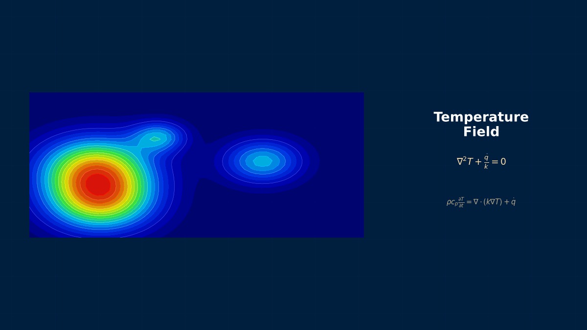
What is the Shape Factor?
Professor, what is the shape factor used for?
It's a concept for reducing 2D or 3D steady-state heat conduction problems to 1D thermal resistance. Using the shape factor $S$,
can be expressed, allowing direct determination of heat dissipation from $\Delta T$. The thermal resistance is $R = 1/(kS)$.
So complex shapes can be aggregated into a single numerical value.
$S$ is a geometric quantity determined solely by shape and boundary conditions, with units of [m] (for 2D problems, [m/m] = dimensionless/unit depth).
Typical Shape Factors
| Shape | $S$ | Applicable Conditions |
|---|---|---|
| Infinite Plate | $A/L$ | Basic form |
| Concentric Cylinders | $2\pi L / \ln(r_2/r_1)$ | Length $L$ |
| Concentric Spheres | $4\pi r_1 r_2/(r_2 - r_1)$ | — |
| Buried Sphere (from surface at depth $z$ in semi-infinite medium) | $4\pi r / (1 - r/(2z))$ | $z > r$ |
| Buried Cylinder (semi-infinite medium) | $2\pi L / \cosh^{-1}(z/r)$ | $z > r$, $L \gg r$ |
| Two Parallel Cylinders | $2\pi L / \cosh^{-1}((d^2-r_1^2-r_2^2)/(2r_1 r_2))$ | Center-to-center distance $d$ |
The formulas for buried spheres and cylinders seem very practical.
They are used in calculating heat dissipation from underground buried pipes, ground heat transfer from building foundations, and geothermal heat pump design. The biggest advantage of shape factors is obtaining rough estimates by hand calculation.
Derivation of Shape Factors
Derived from the solution of Laplace's equation $\nabla^2 T = 0$. For concentric cylinders:
Thus, $S = 2\pi L / \ln(r_2/r_1)$ is obtained.
So you back-calculate the shape factor from the analytical solution.
For shapes without an analytical solution, $S = q/(k\Delta T)$ is calculated numerically using FEM.
Definition and Physical Meaning of Shape Factor
The shape factor S is a dimensionless coefficient expressing heat flow rate in complex shapes as q=SkΔT. Systematized by Carslaw & Jaeger in "Conduction of Heat in Solids" in the 1950s, analytical solutions for over 60 types from buried pipes to spheres and cylinders were compiled as tables.
Computational Methods for the Shape Factor
Numerical Calculation of Shape Factor
How do you find the shape factor for complex shapes?
Solve steady-state heat conduction with FEM and calculate $S$ using the following steps.
1. Set Dirichlet conditions: $T_1$ on the high-temperature surface, $T_2$ on the low-temperature surface.
2. Set $k = 1$ W/(m K) (for simplification).
3. Run the analysis and obtain the total heat flow rate $q$ on the high-temperature (or low-temperature) surface.
4. Calculate $S = q / (k \cdot \Delta T) = q / (T_1 - T_2)$.
Setting $k = 1$ is to make the calculation easier, right?
Yes. Since $S$ is a geometric quantity independent of $k$, the value of $k$ does not affect the result.
Mesh Convergence Verification
Since the shape factor is an integral quantity (total heat flow rate), local mesh sensitivity is small, but convergence verification is necessary for complex shapes.
| Mesh Level | Number of Elements | $S$ | Error |
|---|---|---|---|
| Coarse | 1,000 | 15.2 m | — |
| Medium | 10,000 | 15.8 m | 3.9% |
| Fine | 100,000 | 15.9 m | 0.6% |
| Very Fine | 1,000,000 | 15.9 m | 0.0% |
Integral quantities converge relatively quickly.
Integral quantities of temperature converge faster than local stress values. Often, practical accuracy is achieved even with 10,000 elements.
Superposition Principle
Since shape factors are for linear problems, superposition is possible. For multiple heat sources, shape factors from each source can be summed. Also, using symmetry conditions can reduce computational load.
So you can model half using a symmetry plane and then double the $S$, right?
Exactly. For a buried cylinder in the ground, treating the ground surface as a symmetry plane (adiabatic surface) allows reducing the problem from a semi-infinite medium to a finite domain.
How to Use the Analytical Solution List for Shape Factors
The shape factor for a buried pipe in the ground (diameter D, depth z, length L) is S=2πL/ln(4z/D) (when z>>D). For example, for a Tokyo water pipe with D=100mm, z=1m, L=20m, S≈27m; with soil k=1.5 W/m·K, a heat flow rate of q≈243W per ΔT is obtained—a practical calculation.
Shape Factor in Practice
Heat Dissipation Calculation for Buried Pipes in Ground
Where is the shape factor most commonly applied?
Calculating heat dissipation from buried pipes in the ground. The temperature field in the ground can be treated as a semi-infinite medium, and shape factor formulas can be used directly.
Calculation Example
A steam pipe (outer diameter 114.3mm, insulation outer diameter 214.3mm) is buried at a depth of 1.5m from the ground surface. Ground temperature 15°C, insulation outer surface 80°C. Soil $k_{\text{soil}} = 1.5$ W/(m K).
184W of heat dissipation per meter.
For a 100m pipe, that's 18.4kW of heat loss. This is converted to annual energy costs to perform economic optimization of insulation thickness.
Ground Heat Transfer from Building Foundations
Ground heat transfer from slab-on-grade (concrete floor on ground) is also regulated by shape factor-based calculations in ISO 13370.
| Parameter | Impact |
|---|---|
| Foundation Area/Perimeter Ratio | Larger ratio means less heat dissipation to ground |
| Insulation Placement | Insulation at the foundation perimeter is most effective |
| Soil $k$ | Sand 1.5, Clay 1.0, Peat 0.5 W/(m K) |
So larger buildings have an advantage.
Since area scales with $L^2$ and perimeter scales with $L$, larger buildings have a larger area per perimeter, making the impact of ground heat transfer relatively smaller.
References for Shape Factors
A comprehensive list of shape factors is found in Incropera's "Fundamentals of Heat and Mass Transfer" Table 4.1, or in the Appendix of Bejan's "Heat Transfer." For special shapes, Hahne & Grigull's literature is extensive.
For shapes not covered in textbooks, we have to rely on FEM.
Exactly. Once $S$ is obtained via FEM, it can be stored as a design formula in a database for future hand calculations.
Related Topics
Experience the theory firsthand with the interactive simulator for this field
All Simulators