Radiation Heat Exchange between Gray Bodies
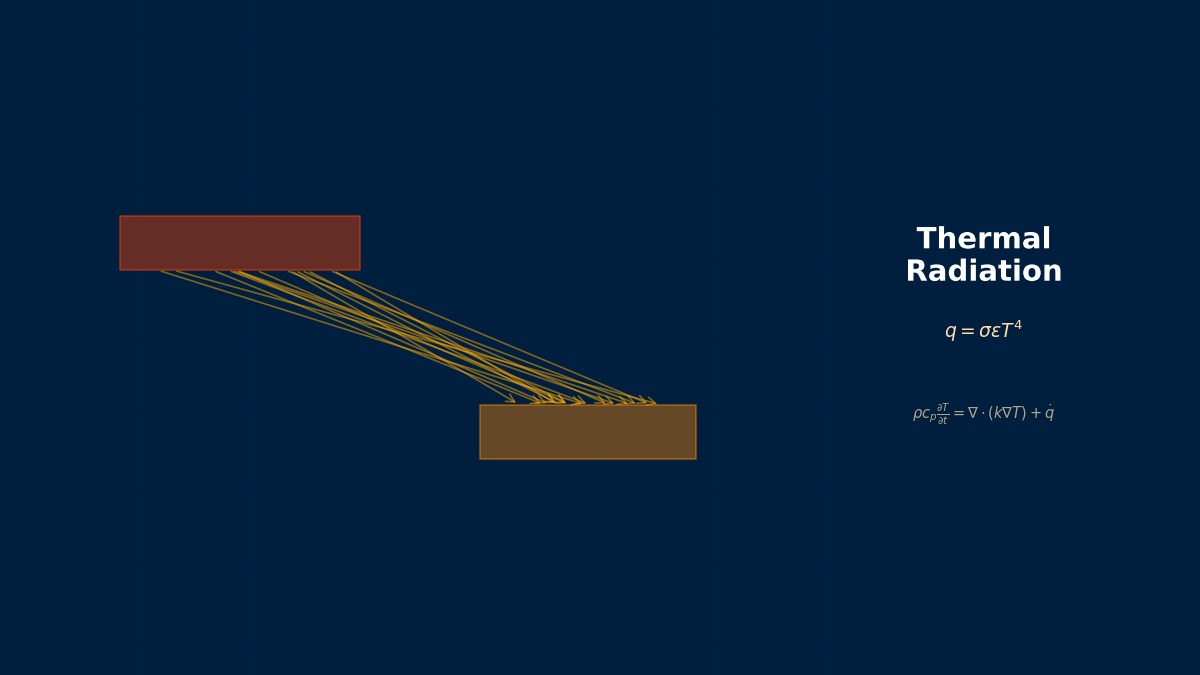
Theoretical Basis of Gray Body Radiative Exchange
The Three Assumptions It Rests On
The standard model for radiative exchange between surfaces — enclosure theory for gray, diffuse surfaces — is built on three assumptions: (1) gray, meaning the radiative properties do not depend on wavelength (for the limits of that, see Kirchhoff's law); (2) diffuse, meaning emission and reflection do not depend on direction; and (3) each surface is isothermal and radiates uniformly. Swallow those three and radiative exchange among any number of surfaces collapses into linear algebra — an exceptionally cost-effective piece of engineering theory. Read the other way round, it is also the list of assumptions to suspect when the result fails to match measurement.
View Factors — The Geometric Vocabulary
The fraction of radiation leaving surface \( i \) that arrives directly at surface \( j \) is the view factor (configuration factor) \( F_{ij} \). It is purely geometric, and two identities always hold.
$$ A_i F_{ij} = A_j F_{ji} \;\;(\text{reciprocity}), \qquad \sum_j F_{ij} = 1 \;\;(\text{summation rule, closed enclosure}) $$
These two equations serve directly as check formulas for computed view factors. A view factor set that violates the summation rule leaks energy (or creates it), so verification of a radiation analysis always starts here.
The Radiation Resistance Network — The Complete Two-Surface Solution
Exchange between gray surfaces is easiest to see through the electrical circuit analogy. Assign each surface a surface resistance \( (1-\varepsilon)/(\varepsilon A) \) and each pair a space resistance \( 1/(A_1 F_{12}) \); the net exchange in a two-surface enclosure is then
$$ Q_{12} = \frac{\sigma (T_1^4 - T_2^4)}{\dfrac{1-\varepsilon_1}{\varepsilon_1 A_1} + \dfrac{1}{A_1 F_{12}} + \dfrac{1-\varepsilon_2}{\varepsilon_2 A_2}} $$
For large parallel plates (\( F_{12}=1, A_1=A_2 \)) this reduces to \( q = \sigma(T_1^4 - T_2^4)/(1/\varepsilon_1 + 1/\varepsilon_2 - 1) \), and for a small body in a large enclosure the resistance on the surrounding side vanishes, leaving \( Q = \varepsilon_1 A_1 \sigma (T_1^4 - T_2^4) \) — the familiar working formulas are all special cases of this one network. The circuit intuition that surface resistance grows as ε shrinks explains, with nothing added, why low-emissivity surfaces such as polished metal and thermal shields work as well as they do.
Computing Multi-Surface Systems
The Radiosity Method — Standard Solution for N Surfaces
Once there are more surfaces, you solve a linear system for the radiosity \( J_i \) of each surface — its total outgoing radiation, emitted plus reflected.
$$ J_i = \varepsilon_i \sigma T_i^4 + (1-\varepsilon_i) \sum_j F_{ij} J_j $$
Temperature-specified and flux-specified surfaces can be mixed freely (an adiabatic or reradiating surface is just the special case \( q=0 \)), and the net flux on every surface follows once the system is solved. The "S2S" (surface-to-surface) model in CFD and FEM tools is this implementation. Numerically, the star of the show is not the equation system but the computation of the view factor matrix: N surfaces require \( N^2 \) geometric integrals including blockage tests, and that is what governs both cost and accuracy.
Computing and Verifying View Factors
| Method | Character |
|---|---|
| Analytic formulas and charts | Standard geometries: parallel plates, perpendicular surfaces, coaxial cylinders. The benchmark for hand verification |
| Area integration (numerical quadrature) | General geometries of moderate size. Blockage testing is the crux of the implementation |
| Hemicube or ray tracing | The standard for large, complex geometries. Resolution (ray count, hemicube resolution) is the accuracy parameter |
| Monte Carlo | The most general (specular and transmitting behaviour come naturally). The price is statistical noise |
Whichever method produced it, subject the resulting matrix to a compliance check against the summation and reciprocity rules. Tools normally offer an option to normalise the rows so the summation rule holds, but a large pre-normalisation error (a row sum below 0.95, say) signals insufficient rays or resolution — normalising merely hides it.
Designing the Surface Subdivision — Protecting the Isothermal Assumption
Assumption (3), that each surface is isothermal, translates into a meshing rule: never treat a surface with a large temperature gradient as a single patch. Model a long cooling fin as one surface and the difference between root and tip is flattened out, so the radiated heat comes out wrong. Subdividing too finely, on the other hand, makes the view factor computation explode, so the working guideline is to split at a granularity that keeps the expected temperature difference within a few tens of K. The clustering setting in S2S — bundling several mesh faces into one radiating surface — is exactly the knob for this trade-off.
Guidance for Practical Use
A Hand Calculation — Getting a Feel for the Numbers
I never quite get a feel for how much radiation matters compared with convection.
Let us do one. Take parallel plates facing each other at 500 K and 300 K, both with \( \varepsilon = 0.8 \). Then \( \sigma(T_1^4 - T_2^4) = 5.67\times10^{-8} \times (6.25\times10^{10} - 8.1\times10^{9}) \approx 3080 \) W/m², and the denominator is \( 1/0.8 + 1/0.8 - 1 = 1.5 \), so \( q \approx 2050 \) W/m². That is a heat flux on a par with forced convection. Inside an electronics enclosure, by contrast, where both surfaces sit within about ±20 K of room temperature, radiation gives a few tens of W/m² — the same order as natural convection. Because of the nonlinearity of the difference of fourth powers of absolute temperature, whether radiation matters changes dramatically with temperature level. Get into the habit of settling the question with that two-line hand calculation.
Designing Radiation Shields
Insert a single low-ε shield between two surfaces and the radiation resistances add in series, roughly halving the heat flow (for equal ε, N shields give a factor \( 1/(N+1) \)). Multi-layer insulation (MLI) is this principle taken to its limit: spacecraft achieve effective emissivities around 0.01 with several tens of layers. Two design cautions. First, the shielding effect is more dramatic the smaller ε is, because surface resistance dominates. Second, in hardware, contact conduction through spacers and seams plus edge leakage degrade the theoretical value badly — MLI routinely delivers a fraction of its theoretical performance, so design work uses measured effective emissivities.
Linearising Radiation — Folding It into Thermal Networks and Transients
When temperature differences are small, radiation can be linearised and handled in the same form as convection: \( h_r = 4\varepsilon\sigma T_m^3 \), where \( T_m \) is the mean temperature. Near room temperature this gives \( h_r \approx 5\varepsilon \) W/m²K straight away — the same order as natural convection. It is the standard trick for adding radiation cheaply to a thermal resistance network or a 1D analysis, but where the temperature difference is large (a ratio above about 1.5) the linearisation error is no longer negligible, so keep the fourth power or update it iteratively.
Handling It in the Tools
Key Settings by Tool
| Tool | Model | Key points |
|---|---|---|
| Ansys Fluent | S2S (plus DO and others) | Cluster size (faces per cluster) is the main accuracy/cost knob. Confirm the summation rule is satisfied |
| Ansys Mechanical | Radiosity (surface-to-surface radiation) | Define the enclosure explicitly and state the ambient temperature seen through any opening |
| STAR-CCM+ | S2S, ray tracing | Treat convergence in patch resolution and ray count on a par with mesh convergence |
| Spacecraft and vehicle thermal tools (ESATAN, TAITherm and similar) | Monte Carlo view factors plus a thermal network | Statistical convergence in ray count; model MLI with an effective emissivity |
| OpenFOAM | viewFactor (S2S), fvDOM | Watch the face-agglomeration settings of the viewFactor generation utility |
Modelling Open Systems — Do Not Forget the Virtual Surface
Enclosure theory presumes a closed space. For open housings and outdoor equipment the standard device is to close the enclosure by stretching a virtual black surface at ambient temperature across the opening; forget it and the summation rule breaks, so heat disappears. In some tools an "environment temperature" setting plays that role automatically, but what that ambient temperature represents — sky, ground, or room wall — is a physical decision for the analyst. Outdoors, how the effective sky temperature is treated (equivalent to roughly 10 to 20 K below air temperature on a clear night) drives the result.
Frontiers
Extensions to Specular and Spectral Behaviour
Beyond gray diffuse lie more precise models: partially specular reflection (splitting diffuse and specular, then generalising via the BRDF), wavelength band splitting (non-gray), and formulations that include polarisation. GPU-accelerated ray tracing is making Monte Carlo spectral computation practical even on the large models that once had to settle for gray diffuse, and adoption is advancing in headlamp, optical system and high-temperature furnace design. The standard practical strategy is hierarchical: capture the whole picture with gray diffuse first, then refine only the surfaces the result is sensitive to.
Coupling with Participating Media (Gases and Particles)
Where combustion gases (CO₂, H₂O), soot or sprays intervene, absorption, emission and scattering by the medium are added to the surface-to-surface exchange, and the subject becomes the pairing of a radiative transfer solver (DO/DOM, P1, Monte Carlo) with a non-gray gas model (WSGG, SLW, k-distribution). Surface S2S theory makes the approximation "the medium is transparent" explicit — recognising where that approximation fails, as it does in furnaces and engine cylinders, is the starting point for model selection.
Near-Field Radiation — Outside the Theory
When the gap between surfaces approaches the wavelength of thermal radiation (~10 μm), tunnelling of evanescent waves carries heat at rates orders of magnitude above the blackbody limit — near-field radiation. Measurements are advancing in MEMS, thermophotovoltaics and nano-gap devices, and a design theory is forming for a scale at which conventional view factor theory simply does not apply. For a macro-scale designer it is knowledge of a boundary: at micrometre gaps, different physics takes over.
Troubleshooting
Symptoms, Causes, and Fixes
| Symptom | Likely cause | Fix |
|---|---|---|
| The energy balance does not close | Summation rule violated by the view factors; the virtual surface at an opening was forgotten | Check row sums and reciprocity of the F matrix. Add a surrounding surface across the opening |
| The result keeps moving as resolution is raised | Ray count, clustering or surface subdivision not converged | Run a convergence study on radiation resolution just as you would on mesh |
| Temperatures around low-ε surfaces are unstable or non-physical | Multiple reflections converge poorly as ε→0 | Put a realistic floor on ε (0.02 to 0.05) and strengthen the iterative convergence settings |
| Shields or MLI do not deliver the measured benefit | Contact conduction, edge leakage, penetrations | Remodel with an effective emissivity; add the conduction paths to the thermal network |
| Radiation from a large surface looks wrong (fins and similar) | The isothermal-surface assumption has broken down | Subdivide the surface along the temperature gradient |
| Disagreement with measurement although the setup looks right | ε for the wrong surface condition; non-gray behaviour (hot source) | Go to the Kirchhoff article for band separation and checking the source of ε |
A Verification Pattern for Radiation Analyses
Radiation analysis strikes me as hard to verify. Is there a standard procedure?
Three items make it routine. (1) Compare against analytic solutions — pull a two-surface subset out of the model and check it against the parallel-plate and concentric-cylinder formulas (a home-grown equivalent of the radiation entries in the NAFEMS benchmarks). (2) Check the matrix identities — record the residuals of the summation and reciprocity rules as numbers. (3) Resolution convergence — double the ray count or cluster count and watch the target quantity. All three work whatever the solver is. And when you do compare with measurement, suspect the basis of ε (the surface condition) first: more than half of the discrepancies in radiation analysis come down to the ε input rather than the model.
Related: Kirchhoff's law, index of radiation heat transfer articles, NAFEMS T4 (a pattern for verifying boundary conditions).
Feel the theory hands-on with the interactive simulators in this field
Simulator LibraryRelated Fields
detail
error