NAFEMS T4: Heat Conduction with Convective Boundary Condition
Benchmark Specification and Theoretical Background
What the NAFEMS Benchmarks Are
The standard benchmark collection published by NAFEMS (the UK-founded association for analysis engineers) supplies small verification problems that come with reference solutions, and it is the common language of solver verification worldwide. T4 is its representative heat-conduction problem, designed so that in 1 problem you can confirm whether the convective boundary condition (type 3, the Robin condition) has been implemented and set up correctly. It is the standard first thing to solve when a new solver is introduced, when a version is upgraded, or when teaching thermal analysis.
The T4 Problem Setup
Steady 2-D heat conduction on a rectangular plate 0.6 m wide and 1.0 m high.
| Item | Value |
|---|---|
| Thermal conductivity | \( k = 52 \) W/(m·K) |
| Bottom edge (y=0) | Prescribed temperature \( T = 100 \)°C |
| Left edge (x=0) | Adiabatic (symmetry) |
| Right and top edges | Convection: \( h = 750 \) W/(m²·K), ambient temperature \( T_\infty = 0 \)°C |
| Evaluation point E (x=0.6, y=0.2) | Reference solution \( T_E = 18.3 \)°C |
The governing equation is the Laplace equation \( \nabla^2 T = 0 \), and the convective edges carry the boundary condition \( -k\,\partial T/\partial n = h\,(T - T_\infty) \).
Why It Counts as a Good Verification Problem
It is only heat conduction in a rectangle, isn't it? What can a problem this simple really verify?
It is nastier than it looks. Start with the Biot number — \( Bi = hL/k = 750\times0.6/52 \approx 8.7 \). Convection is stronger than conduction, so the temperature field develops steep gradients near the boundaries. On top of that, point E sits close to the bottom-right corner where the prescribed-temperature edge (100°C) meets a convective edge, exactly where the gradient is steepest. A coarse mesh drifts by several °C with no effort at all. And because a convective boundary is implemented as an integral over surface elements, a wrongly applied h, a wrongly oriented face or a mis-set ambient temperature shows up in the number immediately. Dirichlet, adiabatic and Robin: all 3 boundary types in 1 problem — as a detector of setup mistakes it is beautifully designed.
Procedure and Convergence Check
The Standard Procedure
- Element choice — quadratic quadrilaterals with 8 nodes (2nd-order) are recommended. 1st-order elements will solve it too, but converge more slowly
- Mesh series — for example the 3 levels 6×10, 12×20 and 24×40 (refinement ratio 2). Choosing divisions that place point E on a node removes any argument about interpolation error
- Boundary settings — 100°C on the bottom edge, convection on the right and top edges (h=750, T∞=0°C), and nothing at all on the left edge (adiabatic by default)
- Evaluation — tabulate \( T_E \) for every level and confirm convergence towards the reference value of 18.3°C
Acceptance Criteria
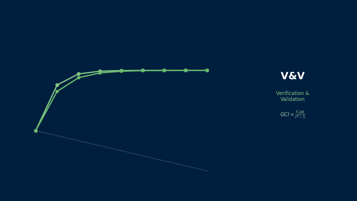
On a fine mesh of 2nd-order elements \( T_E \) converges to 18.2–18.3°C. The practical pass criterion is monotone convergence to within ±0.5% (±0.1°C) of the reference value. Solving 1 mesh level and signing off with "we got 18.6°C, near enough" falls short as verification: you have only solved T4 once you can show the mesh-convergence trend itself. Take it as far as an order-of-convergence estimate (GCI) and it becomes an in-house verification template exactly as it stands.
Keeping the Discretised Convective Boundary in Mind
In the finite element method a convective boundary condition is implemented as integrals over the boundary elements: \( \int_\Gamma h\,N_i N_j\,dS \) enters the stiffness matrix and \( \int_\Gamma h\,T_\infty N_i\,dS \) enters the load vector. In other words h is a quantity that attaches to a face, so applying it to nodes or volumes by mistake, selecting the wrong faces, or confusing the front and back of an element all appear directly in the temperature field. If T4 reproduces the reference value, that is proof that this whole boundary-implementation chain is correct.
Putting It to Work in Practice
Use as an Acceptance and Regression Test
The practical value of T4 lies not in "solve it once and be done" but in a reference standard you use again and again: acceptance testing of a new solver or a new version (has the boundary handling changed in the update?); equivalence checks when migrating the analysis environment; a day-1 exercise for new engineers, who get hands-on with all 3 boundary types at once; and sanity-checking input templates. Script the input file together with its expected value (18.3°C±0.1) and every environment update can be regression-checked in minutes.
Pitfalls of Units and the Temperature Datum
T4 is defined in degrees Celsius, but since the problem is linear and free of radiation, absolute temperature gives the same answer (with T∞=0°C=273.15 K and 100°C=373.15 K you obtain \( T_E = 291.45 \) K = 18.3°C). Mixing this up with the solver's default temperature unit is instantly fatal, however — "I entered 0 for T∞ but the unit was K (= −273°C)" is the classic mistake, and it is the first thing to suspect when the result swings far to the negative side. In non-SI unit systems (mm-based) the conversion of h (W/m²K → mW/mm²K) also needs care.
How to Extend It — Staged Verification Starting from T4
Once T4 passes, the same model lets you widen the verification scope step by step: add temperature-dependent properties and check the iterative convergence of nonlinear heat conduction; make it transient and verify the time integration (a transient from an initial temperature of 0°C); make the convective h temperature-dependent and verify boundary nonlinearity; split the solid into 2 materials and verify interface continuity. A 1-step extension from a problem that has a reference solution is the shortest route to separating bugs from physics in a complex model.
How to Set It Up Tool by Tool
Names for the Convective Boundary Condition
| Tool | Convective boundary setting | Note |
|---|---|---|
| Abaqus | *FILM (film coefficient h and sink temperature on a surface) | Applied to a surface definition. Units are managed dimensionlessly across the whole input |
| Ansys Mechanical | Convection load (Film Coefficient + Ambient Temperature) | SF,,CONV in MAPDL. Check the edge/face selection |
| Nastran (thermal) | CONV + PCONV for the convective boundary, prescribed temperature via the SPC equivalent | Note that the thermal boundary card system is separate from the structural one |
| COMSOL | "Convective heat flux" under the heat flux boundary (h and T_ext) | The out-of-plane thickness in 2D does not affect the result (linear and steady) but stating it explicitly is recommended |
| OpenFOAM | externalWallHeatFluxTemperature (mode: coefficient) | Solid conduction is assembled from the laplacianFoam family plus boundary types |
| In-house and teaching FEM codes | Boundary integral terms implemented by hand | T4 is precisely the right verification problem for that implementation |
Modelling Details That Must Be Aligned
When cross-checking results between tools, align three things: how the value at the evaluation point is taken (nodal value or in-element interpolation); how the midside nodes of 2nd-order elements are treated; and which 2-D formulation is used (no mistaken choice between pure 2-D, unit-thickness plane and axisymmetric). If more than 0.1°C of difference remains between tools on a problem as simple as T4, the cause is almost never physics but these post-processing and formulation differences.
Benchmark Culture Today
The Standard Benchmark Families and Where T4 Sits
The NAFEMS benchmark collection is organised into families — thermal (the T series), linear elasticity (the LE series), free vibration (the FV series) — every one of them designed on the principle that a reference solution exists and a specific capability is targeted. T4 covers the convective boundary, while LE5 covers warping-restrained torsion and LE11 thermal stress: 1 problem, 1 feature is the deliberate simplification. In the language of the ASME V&V standards these belong to code verification, placed ahead of validation against experiment.
Towards Automated Verification Suites
In modern solver development and operation it has become standard to build NAFEMS-style benchmarks into CI (continuous integration) and run them automatically on every code change. On the user side too, a growing number of organisations run an in-house benchmark collection automatically whenever the analysis environment (solver, OS, libraries) is updated and report the differences from the reference values. A lightweight problem like T4 is ideal for this purpose, acting as a safety net that mechanically guarantees the answer does not change when the environment does.
Higher-Precision Reference Solutions
The reference values of the classical benchmarks were produced with the computing resources of their day, and modern high-accuracy computation (hp-FEM, series solutions, extrapolation) has now fixed many more digits. The 18.3°C of T4 is ample for practical work, but if you want a stricter discussion of the order of convergence, a practical approach is to carry alongside it a "working reference value" obtained by Richardson extrapolation of your own ultra-fine mesh solutions.
Troubleshooting
Diagnostic Table for "It Does Not Come Out at 18.3°C"
| Symptom | Likely cause | Fix |
|---|---|---|
| Several °C high or low (moves closer as the mesh is refined) | Plain discretisation error | Confirm convergence with 2nd-order elements plus refinement. Normal behaviour |
| Strongly negative, non-physical values | Mixed temperature units (T∞=0 treated as K) | Check the solver's temperature unit setting |
| Temperatures too high everywhere | Convective edges never set (left adiabatic), or h off by an order of magnitude | Visualise the boundary assignment to confirm it. Check the units behind h=750 |
| Temperature field not symmetric left to right | Adiabatic and convective edges swapped | Re-check the edge mapping (left = adiabatic, right and top = convection) |
| Slightly different values at the evaluation point between tools | Nodal value versus interpolated value, differences in averaging | Make the evaluation point coincide with a node. Standardise the extraction method |
| Convergence oscillates | Unsystematic refinement by an adaptive mesh | Switch to systematic refinement of a structured grid (6×10 → 12×20 → 24×40) |
What a Benchmark Is Really For
I got 18.3°C without trouble! Can I now say our thermal analysis is verified?
What you can claim is that the implementation and setup of steady linear heat conduction with a convective boundary are correct — and even that is a big step. Real projects bring in radiation, temperature-dependent properties, thermal contact resistance and transient effects, so the right picture is to keep stacking up benchmarks feature by feature. My recommendation is to build a matrix of "the features you use" against "the benchmarks you have verified". The blank cells are the features not yet verified in your analysis environment — they show you where the risk lives. T4 is the problem that becomes the 1st row of that table.
Related reading: index of NAFEMS benchmarks, NAFEMS LE5, mesh convergence verification with GCI, forced convection over a flat plate (the physics behind h).
Feel the theory hands-on with the interactive simulators in this field
Simulator LibraryRelated Fields
detail
error