Participating Media Radiation Transfer
Participating Media Radiation Transfer: Theoretical Foundations
What is Participating Media?
Professor, I'm hearing the term "participating media" for the first time. Does ordinary air also affect radiation?
Good question. Symmetric diatomic molecules like nitrogen (N₂) and oxygen (O₂) actually absorb and emit almost no infrared radiation. So air at room temperature is almost "transparent" to radiation.
However, polyatomic molecules like CO₂ and H₂O are a different story. These strongly absorb and simultaneously emit infrared radiation at specific wavelength bands (e.g., 2.7μm, 4.3μm, 15μm bands) corresponding to their molecular vibration frequencies. Media that "interact with radiant energy" like this are called participating media.
I see... but in daily life, we don't feel like air is absorbing infrared radiation, right? In what situations does it become important?
The key points are temperature and scale. At room temperature over a 1m distance, gas radiation is almost negligible. But the story changes completely in situations like these:
- Gas turbine combustion chamber (above 1500°C): Radiation from CO₂ and H₂O in the combustion gases accounts for 30–50% of the heat flux to the walls.
- Industrial furnaces / boilers (1000–1600°C): Radiation becomes the primary mode of heat transfer from the high-temperature gases inside the furnace to the heated objects.
- Large-scale fires: Radiant heat from flames causes fire spread to the surroundings. The contribution of soot particles is significant.
- Atmospheric radiation: The Earth's greenhouse effect itself is an infrared absorption phenomenon by CO₂ and H₂O.
Roughly speaking, in systems where high-temperature gases exist, neglecting radiation can lead to fatal design errors.
What? 30–50% of the wall heat flux is from gas radiation? That can't be ignored... Isn't just the view factor between surfaces enough?
Exactly. For surface-to-surface radiation, you only need to calculate the interaction between surfaces using the view factor $F_{ij}$. But when participating media is present, the medium itself becomes both an emitter and an absorber. Energy increases or decreases each time light passes through the medium. Therefore, you have to solve an integro-differential equation called the Radiative Transfer Equation (RTE).
Radiative Transfer Equation (RTE)
Just hearing "RTE" sounds difficult... What kind of equation is it?
The RTE is an equation that describes "how the energy intensity changes as a light ray travels in a certain direction." In steady state, it looks like this:
Let's organize the meaning of each term:
- $I(\mathbf{r}, \hat{\mathbf{s}})$: Radiative intensity at position $\mathbf{r}$, direction $\hat{\mathbf{s}}$ [W/(m²·sr)]
- $\kappa$: Absorption coefficient [1/m] — How much radiation the medium absorbs
- $\sigma_s$: Scattering coefficient [1/m] — How much radiation the medium scatters
- $I_b = \frac{\sigma T^4}{\pi}$: Blackbody radiative intensity (directional integral of the Planck function)
- $\Phi(\hat{\mathbf{s}}' \to \hat{\mathbf{s}})$: Scattering phase function — Probability distribution of scattering from direction $\hat{\mathbf{s}}'$ to $\hat{\mathbf{s}}$
The left side is "the change in intensity when the ray travels a distance $ds$," and the four terms on the right correspond to "increase due to emission," "decrease due to absorption," "decrease due to scattering to other directions," and "increase due to scattering from other directions."
So each of the four terms represents an increase or decrease. By the way, what makes this equation difficult compared to an ordinary differential equation?
Good point. There are three reasons why the RTE is difficult:
- 7-dimensional problem: 3 spatial dimensions × 2 directional dimensions × 1 wavelength dimension × 1 time dimension. Considering full spectrum and time dependence is enormous.
- Integro-differential equation: The scattering term contains an integral over the entire solid angle $4\pi$, so the solutions for all directions are coupled.
- Nonlinear coupling: Through the emission term $I_b \propto T^4$, it is nonlinearly coupled with the energy equation.
That's why it requires computational cost on par with—sometimes even exceeding—the Navier-Stokes equations.
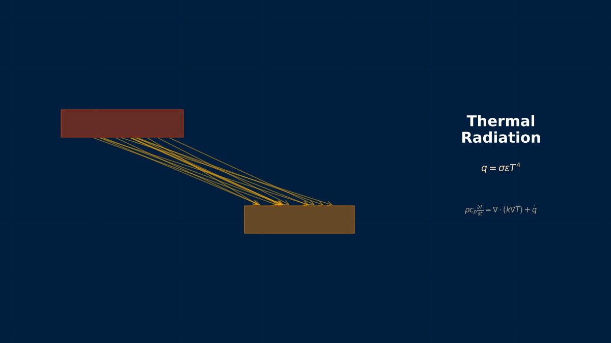
An important relationship derived from the RTE is the radiative source term (the term added to the energy equation):
Here, $G = \int_{4\pi} I \, d\Omega$ is the irradiation, and $\sigma$ is the Stefan-Boltzmann constant ($5.67 \times 10^{-8}$ W/(m²·K⁴)). This term is incorporated as a heat source in the energy equation, coupling radiation with conduction and convection.
Optical Properties and Optical Thickness
I often see the term "optical thickness." What does it specifically mean?
Optical thickness $\tau$ is a dimensionless number representing how much a medium attenuates radiation:
Here, $\beta = \kappa + \sigma_s$ is the extinction coefficient, and $L$ is the characteristic length.
The behavior of the medium changes significantly based on the optical thickness value:
| Optical Thickness $\tau$ | Classification | Physical Behavior | Solution Guideline |
|---|---|---|---|
| $\tau < 0.1$ | Optically thin | Radiation passes through almost unaffected. Contribution of absorption/emission is small. | Can be handled with surface-to-surface radiation + correction for thin gas. |
| $0.1 < \tau < 3$ | Intermediate region | Absorption, emission, and scattering are all important. Most difficult to analyze. | DOM (S4 or higher) or Monte Carlo method required. |
| $\tau > 3$ | Optically thick | Radiation is absorbed and re-emitted over short distances. Behaves diffusively. | P1 approximation or Rosseland diffusion approximation are effective. |
For example, CO₂-rich combustion gas inside a gas turbine combustor is classified as optically thick with $\tau \approx 5\sim10$. On the other hand, for a distance of about 1m in the atmosphere, $\tau \ll 0.1$, making it optically thin.
So the applicable approximation method changes depending on the optical thickness. It makes intuitive sense that the intermediate region is the most troublesome.
Gas Radiation Property Models
Professor, the absorption coefficient of CO₂ and H₂O is completely different depending on the wavelength, right? How is that handled?
That's the most troublesome problem in gas radiation. The actual absorption spectrum of CO₂/H₂O has an extremely complex structure consisting of hundreds of thousands of spectral lines. The absorption coefficient varies by orders of magnitude at wavelength intervals of 0.01 cm⁻¹, so the Line-by-Line (LBL) method, which directly calculates the full spectrum, requires tens to hundreds of thousands of wavelength bands, making it impractical for engineering calculations.
Therefore, in practice, band models or global models like the following are used:
WSGGM (Weighted Sum of Gray Gases Model)
This is the most widely used model. It approximates the radiative properties of a real gas as a weighted sum of $N$ hypothetical gray gases:
Here, $a_{\varepsilon,i}(T)$ are temperature-dependent weighting coefficients, $\kappa_i$ is the absorption coefficient of the $i$-th gray gas, and $pL$ is pressure × path length. $i=0$ corresponds to the "transparent window" with $\kappa_0 = 0$.
The advantage of WSGGM is that engineering sufficient accuracy (within 5% compared to LBL) can be achieved with typically 3–5 gray gases. Representative weighting coefficients, such as those by Smith et al. (1982), are famous and are implemented by default in most CFD solvers.
However, there are also points to note:
- It assumes a gas column with uniform temperature and composition → Modifications are needed for application to non-uniform fields.
- For systems where the CO₂/H₂O molar ratio changes (coal combustion vs. gas combustion), a different coefficient set should be used.
- At high pressures (above 10 atm), coefficients considering pressure broadening effects are necessary.
Are there methods other than WSGGM?
Of course. They are chosen based on the trade-off between accuracy and computational cost:
| Model | Accuracy | Computational Cost | Application Scenario |
|---|---|---|---|
| Line-by-Line (LBL) | Highest (reference solution) | Extremely high | Benchmarking / verification |
| SNB (Statistical Narrow Band) | High | High | Detailed analysis for research purposes |
| WSGGM | Engineering sufficient | Low | Standard for industrial CFD |
| Gray Gas | Low | Lowest | Conceptual design stage |
Soot Particle Radiation
In combustion analysis, "soot" is often discussed. How does radiation change when soot is present?
Soot is a very special entity from a radiation perspective. While gas molecules absorb and emit only at specific wavelength bands, soot particles interact with radiation across the entire continuous spectrum. In other words, soot behaves as an "almost gray" participating medium.
The absorption coefficient due to soot is approximated by:
Here, $f_v$ is the soot volume fraction (typically $10^{-7} \sim 10^{-5}$), $T$ is temperature [K], and $C$ is a constant (approximately 1860 m⁻¹K⁻¹). The total absorption coefficient is summed as $\kappa_{total} = \kappa_{gas} + \kappa_{soot}$.
For example, in a flame containing soot with volume fraction $f_v = 10^{-6}$ and temperature 1500K, $\kappa_{soot} \approx 2.8$ m⁻¹. This is on the same order as the absorption coefficient of CO₂, meaning even a small amount of soot has a massive impact on radiation. In diesel engine combustion chambers or pool fires, radiation from soot often becomes dominant.
Hottel's Gas Radiation Charts — The Origin of Radiation Engineering
Research on radiation in participating media was started in the 1920s by Horace Hottel at MIT. He experimentally compiled the total emissivity of CO₂/H₂O as a function of temperature and pressure×path length (pL) into charts. In an era without digital computers, engineers designed industrial furnaces using only these charts and hand calculations. The WSGGM proposed by Smith, Shen, and Friedman in 1982 was a groundbreaking work that mathematically fitted these Hottel charts into a form implementable in CFD solvers. Even today, the accuracy of WSGGM is often validated against consistency with Hottel charts.
Computational Methods for Participating Media Radiation Transfer
Discrete Ordinates Method (DOM)
How do you actually solve the RTE on a computer? The directional integral seems tough...
The most widely used method is the Discrete Ordinates Method (DOM). The idea is simple: represent the continuous direction $\hat{\mathbf{s}}$ with a finite number of discrete directions $\hat{\mathbf{s}}_m$ ($m=1, \ldots, M$) and solve the RTE for each direction.
In DOM, the RTE is approximated for each discrete direction $\hat{\mathbf{s}}_m$ as follows:
Here, $I_m = I(\mathbf{r}, \hat{\mathbf{s}}_m)$, $w_{m'}$ is the quadrature weight for direction $m'$. The S$_N$ approximation is widely used for selecting directions, where the value of $N$ determines the accuracy:
| $S_N$ Order | Number of Directions (3D) | Accuracy | Computational Cost | Application Guideline |
|---|---|---|---|---|
| S2 | 8 | Low | Low | Preliminary calculations / trend understanding |
| S4 | 24 | Medium | Medium | Minimum line for general industrial calculations |
| S6 | 48 | High | High | Standard detailed analysis |
| S8 | 80 | Very High | Very High | Precise analysis of optically thin regions |
Increasing directions improves accuracy, but also increases computational cost. In practice, is S4 the standard?
Right, in practice, S4–S6 are the most commonly used. S2 has too low directional resolution and is prone to an artificial striped pattern called the ray effect. Conversely, S8 and above cause computational costs to skyrocket, so they are limited to cases where high accuracy is absolutely required.
The strengths of DOM are:
- Can be used regardless of optical thickness (covers optically thin to thick).
- Can handle systems with strong scattering.
- Compatible with unstructured grids.
- Implemented in almost all CFD solvers.
The weakness is that it becomes a system of equations with "number of directions × number of spatial mesh cells," leading to high memory consumption.
P1 Approximation (Spherical Harmonics Method)
What other methods are there besides DOM? I've heard of something called the P1 approximation.
The P1 approximation is a technique in which the angular dependence of the radiative intensity is expanded into a series of spherical harmonics and truncated at the first term:
Here, $G$ is the irradiation and $\mathbf{q}_r$ is the radiative heat flux vector. This reduces the integro-differential RTE to a diffusion-like equation with only two unknowns per spatial point.
The key advantages and disadvantages of P1 are:
- Pros: Extremely low computational cost (only 2 scalar equations per grid cell). Excellent for optically thick media ($\tau > 3$).
- Cons: Very poor accuracy for optically thin and intermediate media. Not suitable for systems with strong directional effects.
For example, in a furnace with uniform high-temperature gas, P1 gives accurate results in seconds. But the same calculation with DOM/S4 might take minutes. The choice depends on whether you need direction-resolved information.
So P1 is the choice when you need speed and the medium is optically thick. Good to know. Are there intermediate options?
Good question. There are several other methods, each with its own niche:
- P3 approximation: Includes higher-order terms for better accuracy than P1, but computational cost is higher.
- Discrete Transfer Method (DTM): A hybrid approach that combines some advantages of DOM and P1. Useful for intermediate optical thickness.
- Monte Carlo method: Probabilistic approach that follows photon trajectories. Extremely flexible and can handle complex geometry and scattering, but requires many samples for low noise.
- Finite Volume Method (FVM) for Radiation: A variant of DOM specifically tuned for unstructured grids.
In modern industrial CFD, DOM/S4 or S6 remains the workhorse for most applications, while P1 is reserved for preliminary studies or optically very thick systems.
Related Topics
Experience the theory with interactive simulators in this field
View Factor Calculator All Thermal Analysis Simulators