Solve a 2x2 linear system A·x=b by the Jacobi iterative method. Adjust the coefficient matrix, right-hand side and iteration count to see whether the system converges or diverges from diagonal dominance and spectral radius, with live views of the error convergence, the iterate trace and the two lines with the iterate sequence.
Parameters
Coefficient a₁₁
Coefficient of x₁ in equation 1 (diagonal entry)
Coefficient a₁₂
Coefficient of x₂ in equation 1 (off-diagonal entry)
Coefficient a₂₁
Coefficient of x₁ in equation 2 (off-diagonal entry)
Coefficient a₂₂
Coefficient of x₂ in equation 2 (diagonal entry)
Right-hand side b₁
Constant on the right side of equation 1
Right-hand side b₂
Constant on the right side of equation 2
Maximum iterations
Stops early once the change drops below 1e-8
Results
—
Solution x₁
—
Solution x₂
—
Iterations
—
Diagonal dominance
—
Spectral radius ρ
—
Converge/Diverge
—
Solution space — two lines and the iterate sequence
The intersection of the two equation lines is the true solution. The iterate sequence starting from (0,0) approaches the intersection when it converges and drifts outward when it diverges.
The Jacobi update. Each unknown x_i is found by dividing by the diagonal entry a_ii, and the right-hand side always uses only the previous iterate x_j^(k).
$$\rho(\text{iteration matrix})\lt 1\quad(\text{holds if diagonally dominant})$$
The convergence condition. The iteration converges if the spectral radius ρ of the iteration matrix is below 1, and diverges otherwise. Strict diagonal dominance always satisfies this condition.
The spectral radius for a 2x2 system. Because Jacobi uses only old values it parallelizes easily, but converges slower than Gauss-Seidel.
What is the Jacobi Iteration Simulator?
🙋
Linear systems are the ones you solve by substitution or elimination, the way they teach in school, right? Is the "Jacobi method" a different way of solving them?
🎓
Yes — a completely different idea. Substitution and determinants are direct methods: they produce the exact answer in one shot. The Jacobi method, by contrast, is an iterative method: you start from some rough guess and nudge it closer to the true answer step by step. This tool starts from x=(0,0). At first that is nothing like the solution, but as you run the update formula again and again, it creeps toward the real answer.
🙋
Isn't creeping up on the answer a roundabout way to do it? Why not just solve it directly in one step?
🎓
For a 2x2 or 3x3 system, sure. But in real CAE work you routinely get a million unknowns. Solving a matrix that huge with a direct method blows up both memory and computation. An iterative method, on the other hand, can exploit the fact that the matrix is sparse — almost all entries are zero — and you can stop the moment you reach the accuracy you need. So for large problems iterative methods take the lead, and Jacobi is their simplest entry point.
🙋
I see. But when I raise a₁₂ on the left, it suddenly turns red and says "Diverge". What just happened?
🎓
Good experiment. Iterative methods have a trap: they do not always converge. The key is diagonal dominance. In each row, when the diagonal coefficient (a₁₁ or a₂₂) is larger in absolute value than the other coefficients in that row, the matrix is "diagonally dominant". When that holds, the Jacobi method always converges. Raise a₁₂ enough to break diagonal dominance and the spectral radius ρ goes above 1 — now the error grows with every iteration, which is exactly divergence.
🙋
The spectral radius ρ is on the results card too. Is that number only about whether it converges?
🎓
Not only that. ρ also sets the speed of convergence. Roughly speaking, the error shrinks by a factor of ρ each iteration. So with ρ=0.3 the digits fall off fast and you converge in a few steps, while with ρ=0.95 it crawls and takes dozens of iterations to reach precision. Look at the "Error convergence" chart below on its logarithmic axis: the slope is exactly log(ρ). The smaller ρ, the steeper the slope down; the closer to 1, the flatter it gets.
🙋
I've heard of a method like Jacobi called "Gauss-Seidel". What is the difference?
🎓
It is the timing of the values used in the update. Within one step, the Jacobi method always uses the previous values on the right-hand side — both x₁ and x₂ are computed from the same old information at once. Gauss-Seidel, the moment it updates x₁, immediately uses that new x₁ when computing x₂. Using fresher information usually makes it converge faster. But because Jacobi computes each component completely independently, it pairs beautifully with parallel computers and GPUs. It is still in active use as the basis of preconditioners and relaxation methods for large sparse matrices.
Frequently Asked Questions
The Jacobi method does not solve a linear system A·x=b directly; instead it improves an approximate solution step by step until it reaches the true answer. Each equation is solved for its diagonal unknown, giving the update x_i^(k+1) = (b_i − Σ_(j≠i) a_ij x_j^(k)) / a_ii. The key feature is that the right-hand side uses only values from the previous step, x^(k). Because every unknown is updated simultaneously, the method parallelizes easily, but it converges more slowly than the Gauss-Seidel method.
The Jacobi method converges when the spectral radius ρ of the iteration matrix (the largest absolute eigenvalue) satisfies ρ<1, and diverges when ρ≥1. For a 2x2 system the iteration matrix is [[0, −a12/a11], [−a21/a22, 0]] and ρ = √|(a12/a11)(a21/a22)|. A sufficient condition is strict diagonal dominance of the coefficient matrix — each diagonal entry larger in absolute value than the other entries in its row (|a11|>|a12| and |a22|>|a21|) — which always guarantees convergence. A non-dominant matrix can still converge if ρ<1, but ensuring diagonal dominance is the safe design choice.
The spectral radius ρ determines not only whether the method converges but also how fast. The error shrinks by roughly a factor of ρ per iteration, so reducing the error tenfold takes about 1/log10(1/ρ) iterations. For ρ=0.3 the error loses a digit every two to three steps, while ρ=0.9 needs more than twenty iterations. On a logarithmic error plot the curve becomes a straight line with slope log(ρ): the smaller ρ, the steeper the descent. As ρ approaches 1 the iteration count grows, and for ρ≥1 the error diverges.
Both are iterative methods, but they differ in which values the update uses. The Jacobi method always uses the previous iterate x^(k) within a single step, whereas the Gauss-Seidel method immediately reuses freshly updated values inside the same step. As a result Gauss-Seidel usually converges faster, and in many cases its spectral radius is roughly the square of the Jacobi one. However, because each Jacobi component is computed independently, the method maps well onto parallel computers and GPUs and is still used as a building block for preconditioners and relaxation methods on large sparse systems.
Real-World Applications
Solver backbone for large CAE analysis: The finite element and finite difference methods used in structural, thermal and electromagnetic analysis ultimately reduce to a huge linear system. Once the unknowns reach hundreds of thousands or tens of millions, a direct method (LU factorization) runs out of memory, so iterative methods are used. The Jacobi method is rarely the final solver itself, but it is embedded as the smoothing step or as a preconditioner inside conjugate-gradient and multigrid methods, where it quickly removes the high-frequency error components.
Parallel computing and GPU acceleration: Each component update in the Jacobi method is fully independent, so every unknown can be computed simultaneously in parallel. This pairs superbly with GPUs and supercomputers of thousands to tens of thousands of cores, with the major advantage that it is not bound to a sequential order the way Gauss-Seidel is. Because it is simple to implement and has a regular communication pattern, it remains widely used as a basic building block of parallel solvers.
Image processing and Poisson equations: Seamless image compositing (Poisson image editing), pressure projection in fluid simulation, and shadow and lighting computation are all problems of solving a Poisson equation, which is a linear system. In these fields Jacobi iteration (or its weighted version) is implemented as a kernel that runs in parallel per pixel on the GPU, supporting real-time processing.
Teaching numerical analysis and understanding algorithms: The Jacobi method is the simplest of the iterative methods, letting you experience the core ideas — convergence conditions, spectral radius, geometric decay of the error — with a minimum of code. Visualizing the behavior on a 2-variable system, as this tool does, makes the sudden divergence when diagonal dominance is broken, and the way ρ governs the speed, intuitive, and provides a foundation for learning more advanced iterative methods.
Common Misconceptions and Pitfalls
The most common misconception is that "an iterative method will always reach the solution eventually if you just run more iterations". An iterative method is only guaranteed to terminate when it converges. If the coefficient matrix is not diagonally dominant and the spectral radius ρ is at least 1, the error is amplified by a factor of ρ at every iteration and you move away from the solution no matter how long you run. Break diagonal dominance in this tool by enlarging a₁₂ or a₂₁ and you can clearly observe that divergence. In practice, when "the iteration does not converge", the first step is to see whether reordering the equations or preconditioning can secure diagonal dominance.
Next is the belief that "diagonal dominance is a necessary condition for convergence". Diagonal dominance is only a sufficient condition, not a necessary one. Even without it, the Jacobi method converges perfectly well as long as the spectral radius satisfies ρ<1. Conversely, if diagonal dominance holds, ρ<1 is guaranteed, so the practical rule is "when in doubt, ensure diagonal dominance and you are safe". This tool displays both the diagonal dominance and ρ, so you can also confirm cases where the two disagree.
Finally, the dismissal that "Jacobi is too slow to be practical". It is true that as a standalone solver it is inferior to Gauss-Seidel and conjugate gradients. But the real value of the Jacobi method lies in its high parallelism and its ability to quickly smooth out high-frequency error. In multigrid methods, the weighted Jacobi method is indispensable as the smoother at each level. And because of the simplicity of using only the diagonal entries, it is also widely used as the most basic preconditioner (Jacobi preconditioning). Rather than discarding it for being slow, the modern approach is to use it as a component in the right place. Note that this tool caps the iterates at ±1e6 on divergence so the numbers never become NaN or Infinity.
How to Use
Enter coefficient matrix values a₁₁, a₁₂, a₂₁, a₂₂ and right-hand side b₁, b₂ in their respective fields.
Set a convergence tolerance (typically 1e-6) and maximum iteration count (50–500).
Click Solve to execute the Jacobi iteration; monitor x₁ and x₂ convergence, diagonal dominance status, and spectral radius ρ.
Worked Example
System: 4x₁ + 0.5x₂ = 9.5; 0.1x₁ + 3x₂ = 6.3. With Jacobi iteration starting from x₁=0, x₂=0, the algorithm updates xₖ₊₁ᵢ = (bᵢ − Σⱼ≠ᵢ aᵢⱼxₖⱼ)/aᵢᵢ. After 12 iterations with tolerance 1e-6: x₁≈2.375, x₂≈2.087. Spectral radius ρ≈0.132 confirms fast convergence; diagonal dominance ratio (|a₁₁|/(|a₁₂|+0)) = 8.0 > 1 validates stability.
Practical Notes
Jacobi converges only when the matrix is strictly diagonally dominant or has spectral radius ρ < 1; use this simulator to verify before deploying in finite-element preconditioners.
For ill-conditioned systems (condition number κ > 1000), increase iteration limit or consider Gauss–Seidel or SOR variants instead.
Real CFD/FEA solvers use Jacobi as a smoother in multigrid; test parameter ranges to understand damping behavior on high-frequency errors.
🎬 Watch it in motion
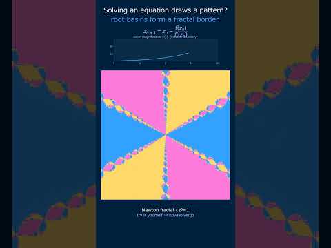
Newton Fractal | which root you reach paints a kaleidoscope #Shorts
Koch Snowflake | the same shape, forever smaller #Shorts
Julia Set | the edge between escape and capture #Shorts
Mandelbrot Set | one tiny formula spins out infinite detail #Shorts