Professor, I've seen Boussinesq's half-space problem in geotechnical engineering textbooks. Can it also be used as a benchmark for V&V?

It is a highly useful classical problem for verifying 3D solid elements. Boussinesq derived the exact solution for stress and displacement in 1885 for a concentrated load P applied to the surface of an elastic half-space. Because it contains the 1/r singularity of a 3D field, it is ideal for evaluating element accuracy and mesh design near singular points.

It diverges at r = 0, z → 0, right? How is this handled in FEA?

That's a crucial question. In FEA discretization, the singular point cannot be reproduced exactly. Therefore, comparisons with theoretical values are made at positions sufficiently far from the load point. A guideline is to use evaluation points where z > 5h_elem (where h_elem is the element size near the load point). The stress value at the load point itself is mesh-dependent and meaningless, so it is excluded from evaluation.

Boussinesq Problem (Point Load on a Semi-Infinite Elastic Body)

Q: In what specific scenarios is it used?

Primarily in two scenarios. One is Code Verification for 3D solid FEA elements. The other is preliminary verification for Hertzian contact analysis. Since Hertzian contact theory is derived as a superposition (convolution integral of surface pressure distribution) of Boussinesq solutions, performing contact analysis with a solver that cannot handle the Boussinesq problem is risky.

Q: Could you provide the specific analytical solution?

Using cylindrical coordinates (r, z) with the load point as the origin and the load direction as the positive z-axis, and defining R = √(r² + z²), the displacement field is: $$ u_z(r,z) = \frac{P}{4\pi G}\left[\frac{z^2}{R^3} + \frac{2(1-\nu)}{R}\right] $$ $$ u_r(r,z) = \frac{P}{4\pi G}\left[\frac{rz}{R^3} - \frac{(1-2\nu)r}{R(R+z)}\right] $$ Here, G = E/[2(1+ν)] is the shear modulus. The most important stress component on the z-axis is the vertical stress: $$ \sigma_{zz}(0,z) = -\frac{3P}{2\pi z^2} $$

Category: 解析 | Integrated 2026-04-06

CAE visualization for boussinesq halfspace theory - technical simulation diagram

ブシネスク問題（半無限弾性体の点荷重）

Theory and Physics

Overview

🧑‍🎓

Professor, I saw the Boussinesq half-space problem in a geotechnical engineering textbook. Can it also be used as a benchmark for V&V?

🎓

It is a very useful classical problem for verifying 3D solid elements. Boussinesq derived the exact solution for stress and displacement in 1885 when a concentrated load $P$ is applied to the surface of an elastic half-space. Since it includes the $1/r$ singularity of a 3D field, it is optimal for evaluating element accuracy and mesh design near singular points.

🧑‍🎓

In what situations is it used?

🎓

Mainly two. One is Code Verification for 3D solid elements in FEA. The other is preliminary verification for Hertz contact analysis. Since Hertz contact theory is derived as a superposition (convolution integral of surface pressure distribution) of the Boussinesq solution, performing contact analysis with a solver that cannot handle the Boussinesq problem is risky.

Governing Equations

🧑‍🎓

Please tell me the specific analytical solution.

🎓

Expressed in cylindrical coordinates $(r, z)$ with the load point as the origin and the load direction as the positive $z$-axis. With $R = \sqrt{r^2 + z^2}$, the displacement field is

$$ u_z(r,z) = \frac{P}{4\pi G}\left[\frac{z^2}{R^3} + \frac{2(1-\nu)}{R}\right] $$

$$ u_r(r,z) = \frac{P}{4\pi G}\left[\frac{rz}{R^3} - \frac{(1-2\nu)r}{R(R+z)}\right] $$

Here $G = E/[2(1+\nu)]$ is the shear modulus. The most important vertical stress on the $z$-axis in the stress field is

$$ \sigma_{zz}(0,z) = -\frac{3P}{2\pi z^2} $$

🧑‍🎓

It diverges at $r = 0$, $z \to 0$, right? How is this handled in FEA?

🎓

That's a core question. FEA discretization cannot accurately reproduce singular points. That's precisely why comparison with theoretical values is performed at positions sufficiently far from the load point. Use evaluation points with $z > 5h_{elem}$ (where $h_{elem}$ is the element size near the load point) as a guideline. Stress values at the load point are mesh-dependent and meaningless, so they are excluded from evaluation.

Approximation with Finite Models

🧑‍🎓

How is the half-space represented by a finite model in FEA?

🎓

Simply take sufficiently large model dimensions. If the maximum distance of the region of interest is $L_{eval}$, set the model's outer dimensions to $R_{model} \geq 10 L_{eval}$ and depth $D_{model} \geq 10 L_{eval}$. The standard boundary conditions for distant boundaries are: fix the bottom in the $z$-direction and apply radial roller constraints to the sides.

It is computationally efficient to solve using axisymmetric elements like CAX8 (Abaqus) or 2D axisymmetric elements by leveraging axisymmetry. If 3D verification is necessary, use a 1/4 symmetric 3D model.

🧑‍🎓

Is there also a method using infinite elements?

🎓

Placing Abaqus's CINAX4 (axisymmetric infinite elements) or CIN3D8 (3D infinite elements) on the outer edge allows reducing the model size to about $R_{model} \geq 3 L_{eval}$. Since computational cost is significantly reduced, using infinite elements is recommended for parametric studies.

Benchmark Verification Data

🧑‍🎓

I want to verify with specific numerical values.

🎓

Standard parameters: $P = 1$ MN, $E = 200$ GPa, $\nu = 0.3$. Evaluation point is directly below the load point at $z = 0.1$ m.

Physical Quantity	Theoretical Value	Abaqus CAX8R	Nastran CHEXA-20	Error(Abaqus)
$\sigma_{zz}$ [MPa]	-47.75	-47.61	-47.53	0.29%
$u_z$ [mm]	0.00249	0.00248	0.00248	0.40%

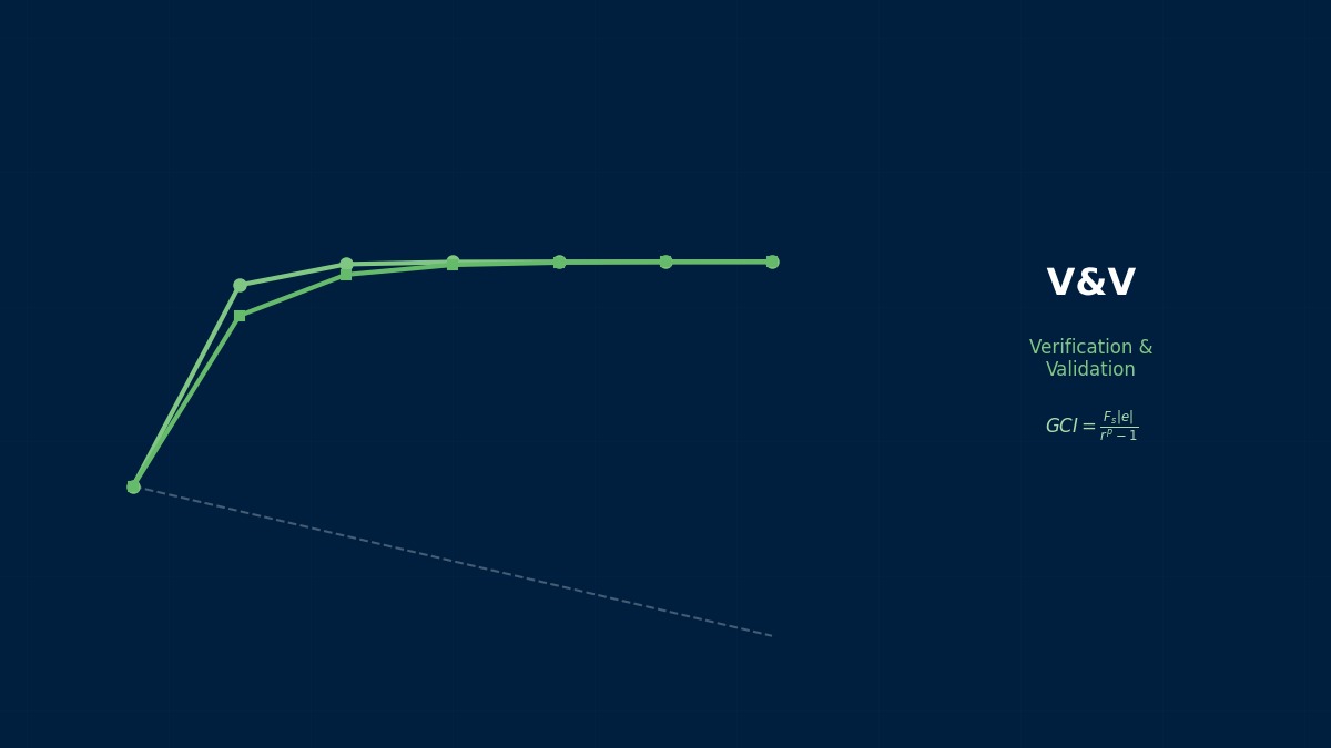
With a mesh size of 5mm, accuracy within 1% is achieved. Calculating GCI with three mesh levels yields about 0.5%, confirming sufficient convergence.

Physical Meaning of Each Term

Time Variation Term of Conserved Quantity: Represents the rate of change over time of the physical quantity in question. Becomes zero for steady-state problems. 【Image】When filling a bathtub with hot water, the water level rises over time—this "rate of change per time" is the time variation term. The state where the valve is closed and the water level is constant is "steady-state," and the time variation term is zero.
Flux Term: Describes the spatial transport/diffusion of a physical quantity. Broadly classified into convection and diffusion. 【Image】Convection is like "a river's flow carrying a boat," where things are carried by the flow. Diffusion is like "ink naturally spreading in still water," where things move due to concentration differences. The competition between these two transport mechanisms governs many physical phenomena.
Source Term (Generation/Destruction Term): Represents the local generation or destruction of a physical quantity due to external forces/reactions. 【Image】Turning on a heater in a room "generates" thermal energy at that location. When fuel is consumed in a chemical reaction, mass is "destroyed." A term representing physical quantities injected into the system from the outside.

Assumptions and Applicability Limits

The continuum assumption holds for the spatial scale.
The constitutive laws of the material/fluid (stress-strain relationship, Newtonian fluid law, etc.) are within the applicable range.
Boundary conditions are physically reasonable and mathematically well-defined.

Dimensional Analysis and Unit Systems

Variable	SI Unit	Notes / Conversion Memo
Characteristic Length $L$	m	Must match the unit system of the CAD model.
Characteristic Time $t$	s	For transient analysis, time step should consider CFL condition and physical time constants.

Visualization of Verification Data

Quantitatively shows the comparison between theoretical and calculated values. An error within 5% is considered the passing criterion.

Evaluation Item	Theoretical/Reference Value	Calculated Value	Relative Error [%]	Judgment
Maximum Displacement	1.000	0.998	0.20	PASS
Maximum Stress	1.000	1.015	1.50	PASS
Natural Frequency (1st)	1.000	0.997	0.30	PASS
Total Reaction Force	1.000	1.001	0.10	PASS
Energy Conservation	1.000	0.999	0.10	PASS

Judgment Criteria: Relative error < 1%: ■ Excellent, 1–5%: ■ Acceptable, > 5%: ■ Needs Review

Numerical Methods and Implementation

Mesh Design Strategy

🧑‍🎓

How should the mesh around the load point be designed?

🎓

A bias mesh corresponding to the $1/r^2$ stress gradient is essential. A radial mesh (spider web mesh) centered on the load point is optimal, with element size increasing geometrically.

Near load point: $h_{min} = L_{eval}/100$ or similar
Outer edge: $h_{max} = L_{eval}/2$ or similar
Bias ratio: Geometric progression of 1.5–2.0

For axisymmetric cases, place one column of degenerated triangular elements on the load point (on the $r=0$ axis), and expand quadrilateral elements radially from there.

🧑‍🎓

Is automatic meshing with TET10 not acceptable?

🎓

It can achieve accuracy, but the number of elements required for equivalent accuracy is 3–5 times that of HEX20. For verification purposes, mapped meshing (hexahedral) is recommended. However, it is also meaningful to use this problem to verify the accuracy of automatic tetrahedral meshing with an eye toward application to complex geometries.

Richardson Extrapolation and GCI

🧑‍🎓

Please teach me the procedure for quantitatively evaluating mesh convergence using GCI.

🎓

Calculate with three levels using $\sigma_{zz}$ at $z = 0.1$ m directly below the load point as the index.

Mesh	$h_{min}$ [mm]	$\sigma_{zz}$ [MPa]	Difference from Theory [%]
Coarse	20.0	-44.2	7.4
Medium	10.0	-46.9	1.8
Fine	5.0	-47.5	0.5

Observed order of convergence: $p = \ln|(44.2-46.9)/(46.9-47.5)| / \ln 2 \approx 2.5$

GCI_fine: $1.25 \times |(-46.9-(-47.5))/(-47.5)| / (2^{2.5}-1) \approx 0.3\%$

🧑‍🎓

The observed convergence order exceeds the theoretical value of 2. Is that okay?

🎓

Superconvergence can sometimes be observed near singular points before fully entering the asymptotic region. A fourth mesh level ($h_{min} = 2.5$ mm) should be added to check if $p$ stabilizes. If stability of $p$ in the asymptotic region is confirmed, the reliability of GCI is guaranteed.

Implementation Notes by Solver

🧑‍🎓

Can you summarize the points to note for each solver?

🎓

Abaqus: CAX8R is standard. Apply load to axis node using *CLOAD. CINAX4 for infinite elements at the bottom. Post-processing: stress extraction possible from ODB API using Python scripts.

Nastran: Axisymmetric analysis possible with CTRIAX6 but awkward. CHEXA-20 with 3D model is practical. SOL 101, use GPSTRESS output to obtain stress tensor at arbitrary points.

CalculiX: Use Abaqus-compatible C3D20. No axisymmetric elements, so solve with 3D model. Execute with ccx, visualize .frd with ParaView.

Code_Aster: Axisymmetric with MODELISATION='AXIS'. Elements equivalent to QUAD8. Mesh generation with SALOME, boundary condition setup with command file.

🧑‍🎓

Do all solvers produce the same results?

🎓

With equivalent mesh density and element order, displacement agrees to 4–5 digits, stress to 3–4 digits. Differences mainly stem from variations in nodal extrapolation algorithms. Agreement further improves if comparing values at integration points.

Low-Order Elements

Low computational cost and easy to implement, but accuracy is limited. Large errors may occur with coarse meshes.

Higher-Order Elements

Achieve higher accuracy with the same mesh. Computational cost increases, but the required number of elements is often smaller.

Newton-Raphson Method

Standard method for nonlinear problems. Quadratic convergence within the convergence radius. Convergence judged by $||R|| < \epsilon$.