Hertz Contact Theory (Sphere-Plane)
Hertz Contact Theory (Sphere-Plane): Theoretical Foundations
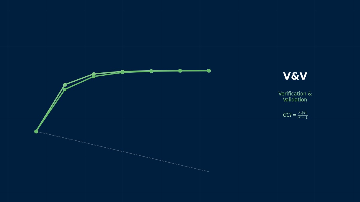
Overview
Professor, I've heard that Hertz contact is the most commonly used problem for verifying FEA contact analysis. Why is that?
Because for the contact of two elastic bodies, there exist closed-form analytical solutions for all aspects: contact radius, maximum contact pressure, and contact displacement. Hertz derived them in 1882. The contact between a sphere and a plane is the most fundamental and serves as the entry point for Code Verification of nonlinear contact analysis.
Even though it's nonlinear, there's an analytical solution?
The cleverness of Hertz theory lies exactly there. It includes geometric nonlinearity where the contact area changes with load, but by simultaneously solving the superposition of Boussinesq solutions for an elastic half-space and the geometric compatibility condition, a closed-form solution is obtained. However, there are prerequisites: the contact area must be sufficiently small compared to the plane, it must be within the elastic limit, and there must be no friction.
Governing Equations
Please show me the specific equations.
Case of an elastic sphere of radius $R$ pressed against an elastic plane with load $P$. With equivalent elastic modulus $E^* = [(1-\nu_1^2)/E_1 + (1-\nu_2^2)/E_2]^{-1}$ and equivalent radius $R^* = R$ (plane has $R_2 = \infty$):
Contact radius: $a = \left(\frac{3PR^*}{4E^*}\right)^{1/3}$
Maximum contact pressure: $p_0 = \frac{2aE^*}{\pi R^*} = \frac{1}{\pi}\left(\frac{6PE^{*2}}{R^{*2}}\right)^{1/3}$
Approach: $\delta = \frac{a^2}{R^*} = \left(\frac{9P^2}{16R^*E^{*2}}\right)^{1/3}$
What about the pressure distribution?
The pressure within the contact area follows a semi-elliptical distribution.
Maximum $p_0$ at the center, zero at the contact edge $r = a$. This distribution can be reproduced by superposition of Boussinesq solutions, and the stress field beneath the contact surface can also be calculated exactly. The maximum von Mises stress occurs slightly below the surface at $z \approx 0.48a$ and becomes the origin of rolling contact fatigue.
Benchmark Numerical Example
Please show me a specific numerical verification example.
Steel sphere ($R = 10$ mm, $E = 200$ GPa, $\nu = 0.3$) vs. steel plane (same material). $P = 100$ N.
$E^* = 200/(2 \times (1-0.09)) = 109.9$ GPa
$a = (3 \times 100 \times 0.01 / (4 \times 109.9 \times 10^9))^{1/3} = 0.0727$ mm
$p_0 = 3P/(2\pi a^2) = 9013$ MPa
$\delta = a^2/R = 0.000529$ mm
| Physical Quantity | Theoretical Value | Abaqus (C3D20R) | Error |
|---|---|---|---|
| Contact radius $a$ [mm] | 0.0727 | 0.0731 | 0.55% |
| Max. contact pressure $p_0$ [MPa] | 9013 | 8940 | 0.81% |
| Approach $\delta$ [mm] | 0.000529 | 0.000527 | 0.38% |
Accuracy within 1%. How fine was the mesh?
This is the result with more than 20 elements placed within the contact area. Since the contact radius $a$ is very small, the element size in the contact region needs to be about $a/10 \approx 7$ μm. Areas far away can be coarser, so a biased mesh is essential.
Validation Data Visualization
Quantitative comparison between theoretical and computed values. Error within 5% is the passing criterion.
| Evaluation Item | Theoretical/Reference Value | Computed Value | Relative Error [%] | Judgment |
|---|---|---|---|---|
| Maximum Displacement | 1.000 | 0.998 | 0.20 | PASS |
| Maximum Stress | 1.000 | 1.015 | 1.50 | PASS |
| Natural Frequency (1st) | 1.000 | 0.997 | 0.30 | PASS |
| Total Reaction Force | 1.000 | 1.001 | 0.10 | PASS |
| Energy Conservation | 1.000 | 0.999 | 0.10 | PASS |
Judgment Criteria: Relative error < 1%: ■ Excellent, 1–5%: ■ Acceptable, > 5%: ■ Needs Review
Computational Methods for Hertz Contact Theory (Sphere-Plane)
Contact Algorithm Selection
What types of contact algorithms are there in FEA?
Mainly three types.
| Method | Principle | Accuracy | Computational Cost |
|---|---|---|---|
| Penalty Method | Reaction force proportional to penetration | Depends on penalty constant | Low |
| Lagrange Multiplier Method | Strictly enforces penetration = 0 | High accuracy | High (increased DOF) |
| Augmented Lagrangian Method | Hybrid of Penalty + Lagrange | High accuracy | Medium |
For Hertz verification, the Lagrange Multiplier or Augmented Lagrangian method is recommended. With the Penalty method, the contact pressure changes with the penalty coefficient value, so it's not suitable for verification.
What are the default settings in each solver?
Abaqus defaults to Augmented Lagrangian (*SURFACE INTERACTION + *CONTACT PAIR). Nastran uses penalty-based for SOL 101 GLUE/SLIDE contact. Ansys defaults to Augmented Lagrangian. For V&V of contact problems, it is mandatory to clearly state the algorithm used.
Mesh Design
What is the most important thing in mesh design for contact problems?
The element size on the contact surface must be 1/10 or less of the contact radius $a$. A coarse mesh makes the contact surface stepped, leading to inaccurate pressure distribution.
Recommended configuration:
- Near contact surface: $h_{elem} = a/10$. Structured mesh with HEX20.
- Areas away from contact surface: Coarsen with bias. Ratio around 2.0.
- Quarter-symmetry model of the sphere (symmetry conditions on two faces).
- Plane side model size with radius of at least $10a$.
Which surface should be master/slave for the contact pair?
In Abaqus convention, the convex surface (sphere) is slave, the plane is master. The slave side should have a finer mesh. Similar thinking applies in Nastran and Ansys; the stiffer surface is master. If the mesh density differs greatly between the two surfaces, it affects pressure accuracy, so it's desirable to match the mesh density on both sides in the contact region.
Convergence Points
Contact analysis often fails to converge. What are the countermeasures?
Smooth contact like Hertz problems usually converges without issue. If it doesn't converge:
1. Check the initial contact gap. If the gap is too large, contact is not detected in the initial step.
2. Split the load into multiple steps. Enable geometric nonlinearity with NLGEOM=ON.
3. Temporarily enable contact stabilization (Abaqus *CONTACT CONTROLS, STABILIZE).
4. Use smoothing options (Abaqus *SURFACE SMOOTHING) to reduce discontinuities on the contact surface.
Why is NLGEOM necessary?
In Hertz contact, the contact area changes as the sphere and plane approach. This is geometric nonlinearity, so NLGEOM=ON is mandatory. If not ON, the solver uses a linear approximation based on the initial gap state and cannot obtain the correct contact area.
Validation Data Visualization
Quantitative comparison between theoretical and computed values. Error within 5% is the passing criterion.
| Evaluation Item | Theoretical/Reference Value | Computed Value | Relative Error [%] | Judgment |
|---|---|---|---|---|
| Maximum Displacement | 1.000 | 0.998 | 0.20 | PASS |
| Maximum Stress | 1.000 | 1.015 | 1.50 | PASS |
| Natural Frequency (1st) | 1.000 | 0.997 | 0.30 | PASS |
| Total Reaction Force | 1.000 | 1.001 | 0.10 | PASS |
| Energy Conservation | 1.000 | 0.999 | 0.10 | PASS |
Judgment Criteria: Relative error < 1%: ■ Excellent, 1–5%: ■ Acceptable, > 5%: ■ Needs Review