MMS: Spalart-Allmaras Turbulence Model
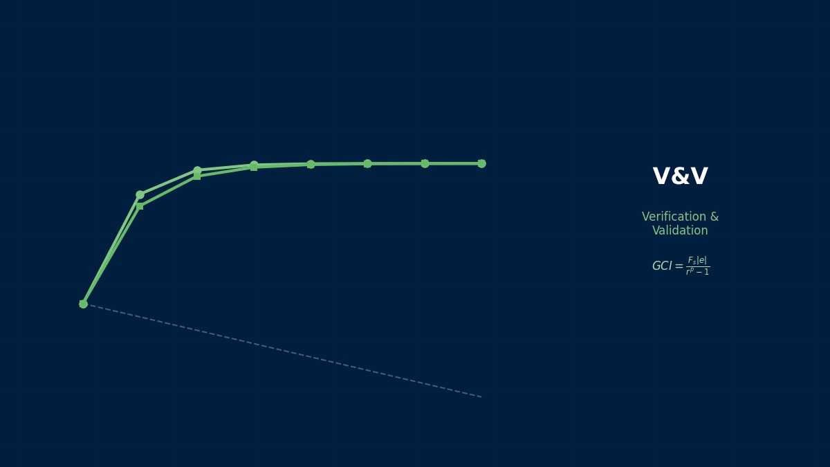
Theory: choose the answer first, then build the source
Overview
Can't we tell whether a turbulence model is implemented correctly by comparing with experiments?
When results disagree with experiments, you can't tell model limitations from program errors; when they agree, a bug may be cancelling another error. Whether the program solves its equations correctly must be checked separately from experiments. That's verification, and the method of manufactured solutions is a powerful way to do it. Choose a solution, substitute it, and add the remainder as a source term; the chosen solution becomes exact. Then just check whether error falls at the theoretical rate under refinement. Equations like SA, with several nonlinear terms, often suffer missing terms or wrong coefficients, which this finds.
A simplified 1D SA equation
From the SA transport equation for ν̃, convection is removed, the destruction function fw is set to 1 and vorticity magnitude to S = 1. Constants: σ = 2/3, cb1 = 0.1355, cb2 = 0.622, cw1 = cb1/κ² + (1 + cb2)/σ = 3.239 (κ = 0.41). Domain 0.1 ≤ y ≤ 1, wall distance d = y, molecular viscosity ν = 0.1 (non-dimensional).
Manufactured solution and observed order
L is the left-hand operator. The source f was derived symbolically (sympy). e_h is the L2 error at spacing h.
The SA model and a culture of verification
The Spalart–Allmaras model, published in 1992 for external aircraft flows, is a one-equation turbulence model widely used for its convenience. But implementations differ in small details, and codes disagreed on the same problem. NASA's Turbulence Modeling Resource collects standard equation forms and verification cases so multiple codes can check convergence to the same answer under grid refinement. Manufactured-solution verification is also used for such implementation checks.
Worked examples
Example: error under grid refinement (second-order central differences, Newton solve)
| Implementation | 20 cells | 40 cells | 80 cells | 160 cells | Observed order |
|---|---|---|---|---|---|
| Correct | 3.40×10⁻³ | 8.38×10⁻⁴ | 2.08×10⁻⁴ | 5.19×10⁻⁵ | 2.02 / 2.01 / 2.00 |
| cb2 term omitted | 1.37×10⁻¹ | 1.34×10⁻¹ | 1.33×10⁻¹ | 1.33×10⁻¹ | 0.03 / 0.01 / 0.01 |
| One-sided face diffusivity | 7.98×10⁻³ | 3.32×10⁻³ | 1.55×10⁻³ | 7.52×10⁻⁴ | 1.26 / 1.10 / 1.04 |
Observed orders come from error ratios between successive grids. The correct implementation converges to the theoretical 2.
Omitting cb2 stops the error falling entirely, but one-sided diffusivity still lets it fall.
They're different kinds of error. Omitting cb2 means the program solves a different equation, so refinement only approaches that other equation's solution and the error stalls near 0.13 — easy to spot. One-sided face diffusivity keeps the equation right but drops discretisation accuracy from second to first order. Refinement still approaches the correct solution, so neither a single-grid result nor comparison with experiment reveals it, but the observed order of 1.04, against a theoretical 2, shows it at a glance. Order verification is valuable because it examines how error falls, not just how large it is.
Verification workflow
- Choose a smooth manufactured solution that exercises every term (no derivative vanishes).
- Derive the source symbolically to avoid transcription errors.
- Compute errors on 3–4 grids and the observed order.
- If the order is off, isolate the cause by removing terms one at a time.
- Disable accuracy-reducing features such as wall functions and limiters during verification.
“Flat-plate friction matched”
An in-house solver with SA matched flat-plate boundary-layer skin friction within a few percent. Yet MMS verification gave an observed order below 2 with the error stalling partway. The cause: the cb2 term's coefficient had not been divided by σ. In a flat-plate boundary layer that term matters relatively little and was hidden among other errors. In separated flows results changed substantially; after the fix they agreed well with another code.
Common mistakes
Mistakes and fixes
| Mistake | Effect | Fix |
|---|---|---|
| Calling experimental agreement verification | Bugs remain | Check order with MMS |
| Solution zeroing some terms | Bugs in those terms missed | Exercise all terms |
| Hand-derived source | Errors in the source itself | Symbolic algebra |
| Grids too coarse | Not in asymptotic range | Use 4+ levels |
| Limiters left on | Order reduced | Disable during verification |
I'd like to learn related topics.
Related pages include an MMS overview, convergence-rate checks, manufactured source terms, MMS for Navier–Stokes and MMS for the Euler equations.
Related Topics
Experience the theory firsthand with the interactive simulator for this field
All Simulators