What equations are used to describe the structural and acoustic sides, respectively?

The structural side uses the standard equations of motion for an elastic body: $$ [M_s]\{\ddot{u}\} + [C_s]\{\dot{u}\} + [K_s]\{u\} = \{F_{ext}\} + [A]\{p\} $$ The term $[A]\{p\}$ on the right side represents the load from sound pressure to the structure, where $[A]$ is the coupling matrix. The acoustic side is governed by the time-domain version of the Helmholtz equation, i.e., the wave equation: $$ \frac{1}{c^2}\ddot{p} - \nabla^2 p = 0 $$

Where do these two systems connect?

They connect through the boundary conditions at the coupling interface. From the acoustic perspective, the normal velocity at the interface must match the structural displacement velocity: $$ \frac{\partial p}{\partial n} = -\rho_f \ddot{u}_n $$ When written in matrix form, the entire coupled system results in an asymmetric equation system: $$ \begin{bmatrix} M_s & 0 \\ \rho_f A^T & M_f \end{bmatrix} \begin{Bmatrix} \ddot{u} \\ \ddot{p} \end{Bmatrix} + \begin{bmatrix} K_s & -A \\ 0 & K_f \end{bmatrix} \begin{Bmatrix} u \\ p \end{Bmatrix} = \begin{Bmatrix} F \\ 0 \end{Bmatrix} $$

音響-構造相互作用

Q: Professor, does acoustic-structure interaction essentially mean that sound and structure mutually influence each other?

Exactly. When a structure vibrates, it pushes the surrounding air or fluid, generating sound waves. Conversely, sound pressure acts as a load on the structure, inducing vibration. This bidirectional coupling is Acoustic-Structure Interaction (ASI).

Q: In what specific scenarios does this become a problem?

Automotive cabin noise is a classic example. Engine vibrations excite the body panels, which then compress and expand the air inside the cabin, creating the sound heard by occupants. Other examples include aircraft fuselage noise transmission, sound insulation design in buildings, and sonar dome design for submarines.

Category: 解析 | Integrated 2026-04-06

Acoustic-structure interaction: vibrating plate coupled to acoustic cavity pressure field with Helmholtz equation and coupling interface conditions — 音響-構造連成系の可視化 — 構造振動モード（左）と音響キャビティ圧力場（中央）の連成界面条件

Overview

🧑‍🎓

先生、音響-構造相互作用って、つまり音と構造が互いに影響し合うってことですか？

Theory and Physics

🎓

That's right. When a structure vibrates, it pushes the surrounding air or fluid, generating sound waves. Conversely, sound pressure acts as a load on the structure, inducing vibration. This bidirectional coupling is Acoustic-Structural Interaction (ASI).

🧑‍🎓

Specifically, in what situations does it become a problem?

🎓

A typical example is vehicle interior noise. Engine vibration excites the body panels, and the panels compress and expand the air inside the cabin, creating the sound heard by occupants. Other examples include aircraft fuselage transmission noise, building sound insulation design, and submarine sonar dome design.

Governing Equations

🧑‍🎓

What equations describe the structural side and the acoustic side, respectively?

🎓

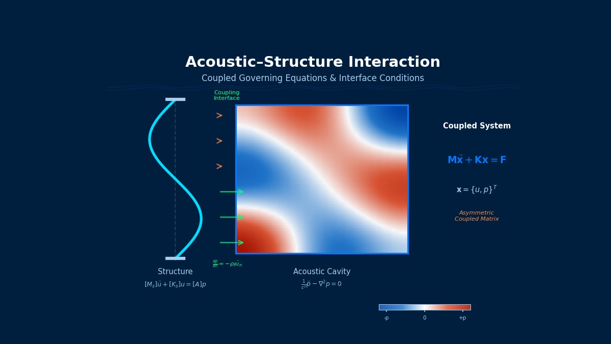
The structural side uses the standard equation of motion for an elastic body.

$$ [M_s]\{\ddot{u}\} + [C_s]\{\dot{u}\} + [K_s]\{u\} = \{F_{ext}\} + [A]\{p\} $$

The term $[A]\{p\}$ on the right side is the load term from sound pressure to the structure, and $[A]$ is the coupling matrix. The acoustic side uses the time-domain version of the Helmholtz equation, i.e., the wave equation.

$$ \frac{1}{c^2}\ddot{p} - \nabla^2 p = 0 $$

🧑‍🎓

Where do these two connect?

🎓

They connect through boundary conditions at the coupling interface. From the acoustic side, the normal velocity at the interface must match the displacement velocity of the structure.

$$ \frac{\partial p}{\partial n} = -\rho_f \ddot{u}_n $$

Writing this in matrix form, the entire coupled system becomes an asymmetric equation system.

$$ \begin{bmatrix} M_s & 0 \\ \rho_f A^T & M_f \end{bmatrix} \begin{Bmatrix} \ddot{u} \\ \ddot{p} \end{Bmatrix} + \begin{bmatrix} K_s & -A \\ 0 & K_f \end{bmatrix} \begin{Bmatrix} u \\ p \end{Bmatrix} = \begin{Bmatrix} F \\ 0 \end{Bmatrix} $$

🧑‍🎓

The asymmetry seems troublesome.

🎓

Indeed. In Nastran, using FLUID elements (CAABSF, CHEXA, etc.) internally assembles this asymmetric coupled system. Abaqus provides *TIE constraints for Acoustic-Structural coupling.

Frequency Domain Formulation

🧑‍🎓

Vibration and noise are often discussed in terms of frequency, right?

🎓

Assuming harmonic response, we can transform to the frequency domain using $\{u\} = \{\hat{u}\}e^{i\omega t}$, $\{p\} = \{\hat{p}\}e^{i\omega t}$.

$$ (-\omega^2 [M_s] + i\omega[C_s] + [K_s])\{\hat{u}\} = \{\hat{F}\} + [A]\{\hat{p}\} $$

$$ (-\omega^2 [M_f]/c^2 + [K_f])\{\hat{p}\} = \rho_f \omega^2 [A]^T \{\hat{u}\} $$

Solving for each frequency allows efficient calculation of the Frequency Response Function (FRF).

🧑‍🎓

With this formulation, it's easier to see which modes are problematic at which frequencies.

🎓

Exactly. Especially when the natural frequency of the structure is close to the natural frequency of the acoustic cavity, coupled resonance occurs, amplifying the sound pressure. The booming problem in vehicle interiors is a classic example.

Practical Points

🧑‍🎓

What should we be careful about when performing analysis?

🎓

First is the acoustic mesh element size. For the maximum analysis frequency $f_{max}$, ensure at least 6 nodes per wavelength are within an element.

$$ h \leq \frac{c}{6 f_{max}} $$

For air with $c = 343$ m/s and $f_{max} = 1000$ Hz, $h \leq 57$ mm. For quadratic elements, it can be slightly coarser, but for linear elements, it's better to adhere to this.

🧑‍🎓

I see, with lower-order elements, a fairly fine mesh is needed. I'm starting to get a clearer picture of the overall concept.

Coffee Break Trivia

"Sound Deforms Structures" – The Phenomenon of Acoustic Radiation Pressure

When learning the theory of acoustic-structural interaction, many people are newly surprised by the fact that "sound pressure exerts force on a structure." In fact, ultrasonic cleaners operate precisely on this principle, where 28–40 kHz sound waves generate microscopic bubbles (cavitation) on the surface of metal parts, physically removing dirt. The sound pressure level can exceed 150 dB. Inaudible to the human ear, yet possessing enough energy to deform metal – the theory of acoustic coupling begins by describing the nature of such "invisible forces" with equations.

Physical Meaning of Each Term

Structural-Thermal Coupling Term: Thermal expansion due to temperature change induces structural deformation, and deformation affects the temperature field. $\sigma = D(\varepsilon - \alpha \Delta T)$. 【Everyday Example】Railroad tracks expanding in summer, narrowing the gaps – a classic case of temperature rise → thermal expansion → stress generation. Warping of electronic circuit boards after soldering is also due to differences in thermal expansion coefficients of different materials. Temperature differences between hot and cold parts of an engine cylinder block generate thermal stress, potentially leading to cracks.
Fluid-Structure Interaction (FSI) Term: Bidirectional interaction where fluid pressure/shear forces deform the structure, and structural deformation changes the fluid domain. 【Everyday Example】Suspension bridge cables vibrating in strong wind (vortex-induced vibration) – wind force shakes the structure, the shaken structure alters the airflow, further amplifying vibration. Blood flow in the heart and elastic deformation of blood vessel walls, and aircraft wing flutter (aeroelastic instability) are also typical FSI problems. One-way coupling may suffice in some cases, but bidirectional coupling is essential for large deformations.
Electromagnetic-Thermal Coupling Term: A feedback loop where Joule heating $Q = J^2/\sigma$ causes temperature rise, and temperature change alters electrical resistance. 【Everyday Example】The nichrome wire in an electric stove heats up (Joule heat) and glows red when current flows – as temperature rises, resistance changes, and current distribution also changes. Eddy current heating in IH cooking heaters and increased sag in power lines due to temperature rise are also examples of this coupling.
Data Transfer Term: Interpolation resolves mesh mismatch between different physical fields. 【Everyday Example】When calculating "feels-like temperature" by combining "temperature data" and "wind data" in weather forecasting, if the observation points differ, interpolation is needed – similarly in CAE coupled analysis, since structural mesh and CFD mesh generally don't match, the accuracy of data transfer (interpolation) at the interface directly affects result reliability.

Assumptions and Applicability Limits

Weak Coupling Assumption (One-Way Coupling): Valid when one physical field affects the other but the reverse is negligible.
Cases Requiring Strong Coupling: Large deformations in FSI, cases with strong temperature dependence in electromagnetic-thermal coupling.
Separation of Time Scales: When characteristic times of each physical field differ significantly, subcycling can improve efficiency.
Interface Condition Consistency: Ensure energy and momentum conservation at the coupling interface is satisfied numerically.
Non-Applicable Cases: When three or more physical fields are strongly coupled simultaneously, monolithic methods may be necessary.

Dimensional Analysis and Unit Systems

Variable	SI Unit	Notes / Conversion Memo
Thermal expansion coefficient $\alpha$	1/K	Steel: ~12×10⁻⁶, Aluminum: ~23×10⁻⁶
Coupling interface force	N/m² (pressure) or N (concentrated force)	Check force balance between fluid and structural sides.
Data transfer error	Dimensionless (%)	Interpolation accuracy depends on mesh density ratio. Aim for below 5%.

Numerical Methods and Implementation

Discretization of Acoustic-Structural Coupling using FEM

🧑‍🎓

How is acoustic-structural coupling handled in FEM? The elements are different for structure and acoustics, right?

🎓

Good question. The structural side uses standard shell or solid elements, and the acoustic side uses acoustic fluid elements with pressure degrees of freedom. At the coupling interface, the displacement DOFs of the structure and the pressure DOFs of the acoustics are coupled.

🧑‍🎓

How is it done in Nastran?

🎓

In Nastran, FLUID elements (acoustic versions of CHEXA, CPENTA, CTETRA) are used, and an ACMODAL surface is defined on the structural face. The coupled system is solved using SOL 108 (Frequency Response) or SOL 111 (Modal Frequency Response).

FEM-BEM Coupling Method

🧑‍🎓

For external radiation problems, the infinite domain is problematic with FEM, right?

🎓

Exactly. For internal problems (closed spaces like vehicle interiors), FEM alone is sufficient, but for external radiation problems, it's combined with BEM (Boundary Element Method). Structural vibration is solved with FEM, and the velocity at the radiating surface becomes the boundary condition for BEM.

The Kirchhoff-Helmholtz integral equation for BEM is as follows.

$$ c(\mathbf{r})p(\mathbf{r}) = \int_S \left[ p(\mathbf{r'}) \frac{\partial G}{\partial n'} - G \frac{\partial p}{\partial n'} \right] dS' $$

Here, $G = \frac{e^{ikR}}{4\pi R}$ is the 3D free-space Green's function.

🧑‍🎓

So BEM doesn't require volume meshes, making it suitable for external problems.

🎓

Yes. Siemens Simcenter 3D (formerly LMS Virtual.Lab) and FFT ASTRA are representative tools for FEM-BEM coupling. HEAD acoustics' ARTEMIS is also boundary element-based.

Statistical Energy Analysis (SEA)

🧑‍🎓

At high frequencies, doesn't the FEM mesh become enormous?

🎓

Sharp observation. In the high-frequency range (roughly above 500 Hz for automobiles), modal density becomes extremely high, making the deterministic FEM approach impractical. That's where Statistical Energy Analysis (SEA) is used.

The basic equation of SEA is power balance.

$$ P_{in,i} = P_{diss,i} + \sum_{j \neq i} P_{ij} $$

$$ P_{ij} = \omega \eta_{ij} (E_i/n_i - E_j/n_j) $$

Here, $\eta_{ij}$ is the coupling loss factor, $n_i$ is the modal density of subsystem $i$, and $E_i$ is the energy.

🧑‍🎓

So the method is chosen based on the frequency band.

🎓

Yes. Low frequency: FEM, High frequency: SEA, Mid-frequency band: Hybrid FE-SEA (supported by Simcenter 3D's Hybrid FE-SEA and Wave). This selection is fundamental to practical vibration-acoustic analysis.

Frequency Band	Method	Representative Tools
Low Frequency (~500 Hz)	FEM / FEM-BEM	Nastran, Abaqus, COMSOL
Mid Frequency	Hybrid FE-SEA	Simcenter 3D, Wave6
High Frequency (500 Hz~)	SEA	VA One (ESI), AutoSEA

Time Domain Explicit Method

🧑‍🎓

What about impact sounds or transient sounds?

🎓

They are solved in the time domain. LS-DYNA supports explicit methods for acoustic-structural coupling and is used for transient analysis of airbag deployment sounds and door closing sounds. Abaqus/Explicit also allows coupling with acoustic elements.