Acoustic Modal Analysis
Theory and Physics
What is Acoustic Modal Analysis?
Professor, does acoustic modal analysis analyze the "vibration of air" rather than the vibration of a structure?
Yes. It finds the natural frequencies and mode shapes of the air inside an enclosed space (passenger compartment, room, duct, etc.). If structural natural vibration is "bone vibration," then acoustic modal is "flesh (air) vibration."
Governing Equation
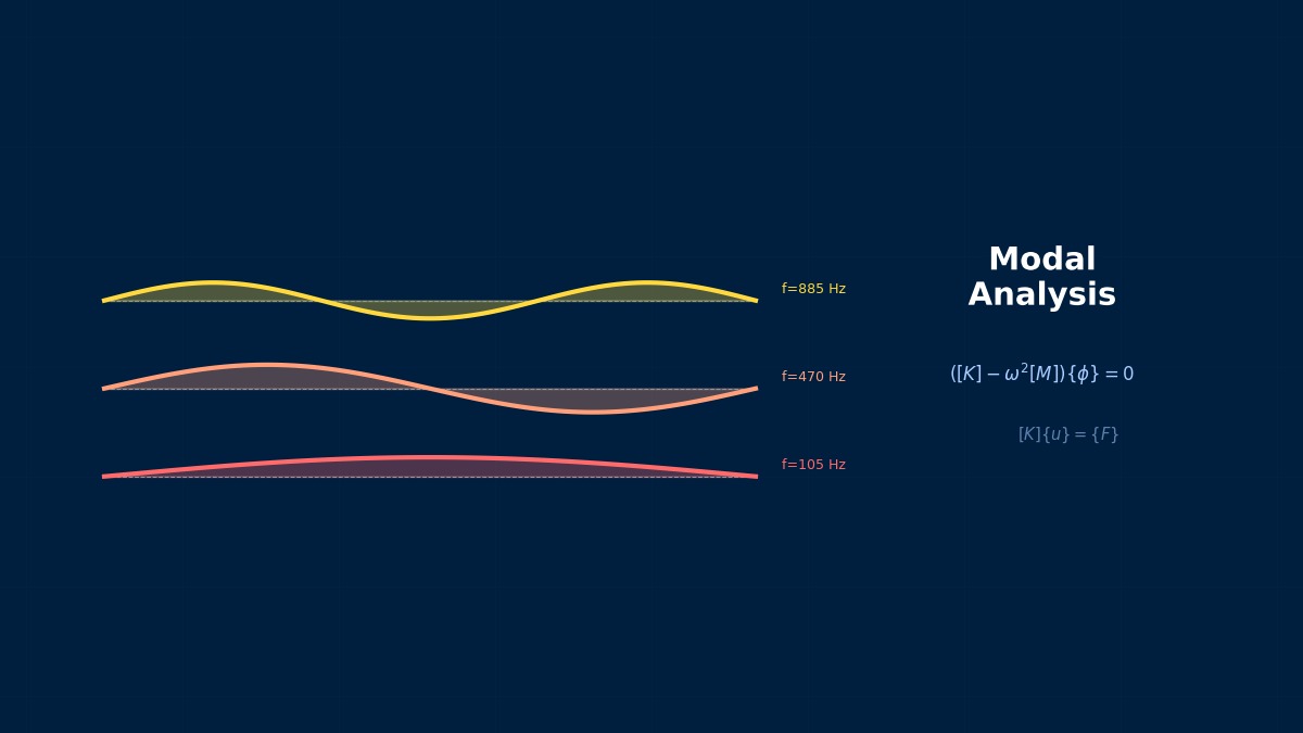
Helmholtz equation for the acoustic field:
$p$ is sound pressure, $c$ is speed of sound. Discretized with FEM:
It has exactly the same form as the structural eigenvalue problem $([K] - \omega^2 [M])\{u\} = \{0\}$!
Correct. The only change is that the unknown is sound pressure $p$ instead of displacement $u$. It can be solved with the same Lanczos method.
Acoustic Modes of a Passenger Compartment
Typical acoustic modes inside an automobile passenger compartment:
| Mode | Frequency | Characteristics |
|---|---|---|
| 1st Longitudinal Mode | 80–120 Hz | Standing wave in front-rear direction |
| 1st Lateral Mode | 200–300 Hz | Left-right direction |
| 1st Vertical Mode | 300–400 Hz | Up-down direction |
The 1st longitudinal mode at 80 Hz is close to engine rotational vibration, right?
The 2nd order (major order) of a 4-cylinder engine is 100 Hz at 3000 rpm. It can potentially resonate with the 1st acoustic mode of the compartment. This is the cause of booming noise. Avoiding this resonance is crucial in NVH design.
Summary
Let me summarize acoustic modal analysis.
Key Points:
- Natural vibration of air in an enclosed space — Eigenvalue problem of the Helmholtz equation
- Same form as structural eigenvalue problem — Solvable with Lanczos method
- Booming noise in passenger compartments — Resonance between acoustic modes and structural vibration
- Foundation of NVH design — Understanding acoustic modes is the first step in noise countermeasures
Reverberation Design in Concert Halls
In 1900, Sabin (Harvard University), the father of acoustics, established the formula for reverberation time T=0.161V/A. This formula was used in the design of Boston Symphony Hall, achieving a reverberation time of 1.8 seconds. Today, calculating indoor acoustic modes with FEM reveals thousands of eigenmodes from 20Hz to 5000Hz, allowing verification of the statistical accuracy of Sabin's formula at the individual mode level.
Physical Meaning of Each Term
- Inertia Term (Mass Term): $\rho \ddot{u}$, meaning "mass × acceleration". Have you ever experienced being thrown forward during sudden braking? That "feeling of being carried away" is precisely the inertial force. Heavier objects are harder to set in motion and harder to stop once moving. Buildings shake during earthquakes because the ground moves suddenly while the building's mass is "left behind". In static analysis, this term is set to zero, which assumes "forces are applied slowly enough that acceleration can be ignored". It absolutely cannot be omitted in impact loads or vibration problems.
- Stiffness Term (Elastic Restoring Force): $Ku$ or $\nabla \cdot \sigma$. When you stretch a spring, you feel a "force trying to return it", right? That is Hooke's law $F=kx$, the essence of the stiffness term. Now a question—an iron rod and a rubber band, which stretches more under the same force? Obviously the rubber. This "resistance to stretching" is the Young's modulus $E$, which determines stiffness. A common misconception: "high stiffness = strong" is incorrect. Stiffness is "resistance to deformation", strength is "resistance to failure"—they are different concepts.
- External Force Term (Load Term): Body force $f_b$ (gravity, etc.) and surface force $f_s$ (pressure, contact force, etc.). Think of it this way—the weight of a truck on a bridge is a "force acting on the entire volume" (body force), while the force of the tires pushing on the road is a "force acting only on the surface" (surface force). Wind pressure, water pressure, bolt tightening force... all are external forces. A common mistake here: getting the load direction wrong. Intending "tension" but applying "compression"—sounds like a joke, but it actually happens when coordinate systems are rotated in 3D space.
- Damping Term: Rayleigh damping $C\dot{u} = (\alpha M + \beta K)\dot{u}$. Try plucking a guitar string. Does the sound continue forever? No, it gradually fades away. That's because vibration energy is converted to heat by air resistance and internal friction in the string. Car shock absorbers work on the same principle—they intentionally absorb vibration energy to improve ride comfort. What if damping were zero? Buildings would continue swaying forever after an earthquake. Since that doesn't happen in reality, setting appropriate damping is crucial.
Assumptions and Applicability Limits
- Continuum assumption: Treats material as a continuous medium, ignoring microscopic heterogeneity
- Small deformation assumption (for linear analysis): Deformation is sufficiently small compared to initial dimensions, stress-strain relationship is linear
- Isotropic material (unless specified otherwise): Material properties are independent of direction (anisotropic materials require separate tensor definition)
- Quasi-static assumption (for static analysis): Ignores inertial and damping forces, considers only equilibrium between external and internal forces
- Non-applicable cases: Large deformation/large rotation problems require geometric nonlinearity. Nonlinear material behavior like plasticity or creep requires constitutive law extension
Dimensional Analysis and Unit Systems
| Variable | SI Unit | Notes / Conversion Memo |
|---|---|---|
| Displacement $u$ | m (meter) | When inputting in mm, unify loads and elastic modulus to MPa/N system |
| Stress $\sigma$ | Pa (Pascal) = N/m² | MPa = 10⁶ Pa. Be careful of unit inconsistency when comparing with yield stress |
| Strain $\varepsilon$ | Dimensionless (m/m) | Note the distinction between engineering strain and logarithmic strain (for large deformation) |
| Elastic Modulus $E$ | Pa | Steel: ~210 GPa, Aluminum: ~70 GPa. Note temperature dependence |
| Density $\rho$ | kg/m³ | In mm system: tonne/mm³ (= 10⁻⁹ tonne/mm³ for steel) |
| Force $F$ | N (Newton) | Unify as N in mm system, N in m system |
Numerical Methods and Implementation
Acoustic Analysis with FEM
What kind of elements are used for the acoustic field in FEM?
Acoustic elements are 1 degree of freedom (sound pressure $p$) elements. Their shape is the same as structural elements (tetrahedron, hexahedron, etc.), but the nodal variable is sound pressure instead of displacement.
| Solver | Acoustic Element | Remarks |
|---|---|---|
| Nastran | CAERO (panel method) or FLUID | Fluid element |
| Abaqus | AC3D4, AC3D8 | Acoustic tetrahedron/hexahedron |
| Ansys | FLUID30, FLUID220 | Acoustic element. Supports structural coupling |
So we mesh the passenger compartment with acoustic elements.
Fill the compartment space with acoustic elements. The wall surfaces (body panels) are structural elements. Define Fluid-Structure Interaction (FSI) at the interface between structure and acoustics.
Structure-Acoustic Coupling
Coupled eigenvalue problem:
$[A]$ is the structure-acoustic coupling matrix.
So structural displacement and acoustic pressure are coupled.
Panel vibration generates sound pressure in the acoustic field, and the sound pressure exerts force back on the structure. Solving this bidirectional coupling allows prediction of the transfer from structural vibration → interior cabin noise.
Summary
Let me summarize the numerical methods for acoustic modal analysis.
Key Points:
- Mesh enclosed space with acoustic elements (sound pressure DOF) — AC3D4/8 (Abaqus), FLUID30 (Ansys)
- Structure-Acoustic Coupling — Displacement and pressure couple at the interface
- Coupled eigenvalue problem — Simultaneous eigenvalues of structure and acoustics
- Core tool for NVH analysis — Prediction of interior cabin noise
Boundary Conditions for FEM Acoustic Modal Analysis
In acoustic modal analysis, air is modeled with potential fluid elements (pressure as unknown), walls are fixed as rigid bodies, and openings are free ends (P=0). The minimum mesh size for finite elements must be 1/6 or less of the wavelength λ at the highest evaluation frequency. For a 1000Hz sound wave in air (λ=340mm), the element size must be 57mm or less.
Linear Elements (1st Order Elements)
Linear interpolation between nodes. Low computational cost but lower stress accuracy. Beware of shear locking (mitigated with reduced integration or B-bar method).
Quadratic Elements (with Midside Nodes)
Can represent curved deformation. Stress accuracy improves significantly, but degrees of freedom increase by about 2–3 times. Recommended when stress evaluation is important.
Full Integration vs Reduced Integration
Full Integration: Risk of over-constraint (locking). Reduced Integration: Risk of hourglass modes (zero-energy modes). Choose appropriately for the situation.
Adaptive Mesh
Automatic refinement based on error indicators (e.g., ZZ estimator). Efficiently improves accuracy in stress concentration areas. Includes h-method (element subdivision) and p-method (order increase).
Newton-Raphson Method
Standard method for nonlinear analysis. Updates tangent stiffness matrix every iteration. Achieves quadratic convergence within convergence radius, but computational cost is high.
Modified Newton-Raphson Method
Updates tangent stiffness matrix using initial value or every few iterations. Cost per iteration is low, but convergence speed is linear.
Convergence Criteria
Force residual norm: $||R|| / ||F_{ext}|| < \epsilon$ (typically $\epsilon = 10^{-3}$ to $10^{-6}$). Displacement increment norm: $||\Delta u|| / ||u|| < \epsilon$. Energy norm: $\Delta u \cdot R < \epsilon$
Load Increment Method
Applies total load not all at once, but in small increments. The arc-length method (Riks method) can trace beyond extremum points on the load-displacement curve.
Analogy for Direct vs Iterative Methods
Direct methods are like "solving simultaneous equations accurately with pen and paper"—reliable but too time-consuming for large-scale problems. Iterative methods are like "repeatedly guessing to approach the correct answer"—the initial answer is rough, but accuracy improves with each iteration. It's the same principle as looking up a word in a dictionary: it's more efficient to open it at an estimated location and adjust forward/backward (iterative method) than to search sequentially from the first page (direct method).
Relationship Between Mesh Order and Accuracy
1st order elements are like "approximating a curve with a ruler"—represented by straight line segments, so accuracy is limited. 2nd order elements are like "flexible curves"—can represent curved changes, dramatically improving accuracy even at the same mesh density. However, computational cost per element increases, so judge based on total cost-effectiveness.
Practical Guide
Practical Application of Acoustic Modes
How are acoustic modes used in practice?
Automotive NVH development is the largest application.
Mesh Requirements
Acoustic element size must be 1/6 or less of the wavelength (for quadratic elements). For $f_{max} = 500$ Hz:
Element size: $0.68 / 6 \approx 0.11$ m = 110 mm.
So acoustic elements are coarser than structural ones.
Because the wavelength of sound waves is longer than that of structural elastic waves, a coarser mesh suffices. However, finer meshes are needed for high frequencies (above 1000 Hz).
Practical Checklist
Related Topics
なった
詳しく
報告