Shock Tube Problem (Riemann Solver)
Theory and Physics
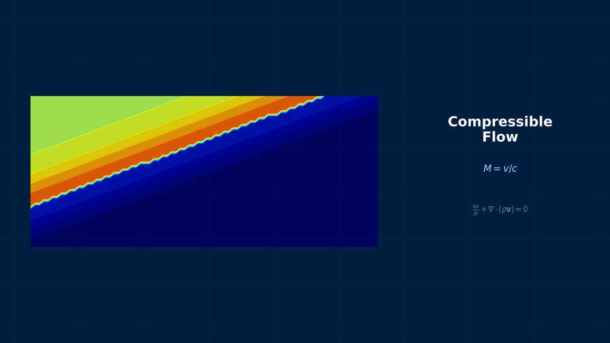
What is the Shock Tube Problem?
Professor, the shock tube problem always appears in CFD textbooks. Why is it so important?
The shock tube problem (represented by the 1D Riemann problem like the Sod problem) is the most fundamental benchmark for evaluating the accuracy and stability of numerical schemes for compressible flow. Because an exact analytical solution is available, it allows for quantitative evaluation of numerical diffusion, overshoot, and shock wave resolution by comparing with the numerical solution.
What exactly is the mechanism for obtaining the exact solution?
It is formulated as an initial value problem for the 1D Euler equations. There is a diaphragm (partition) in the center of the tube, with the left side in a high-pressure state $(\rho_L, u_L, p_L)$ and the right side in a low-pressure state $(\rho_R, u_R, p_R)$. When the diaphragm ruptures, three waves are generated.
1. Leftward traveling expansion wave (rarefaction fan)
2. Central contact discontinuity
3. Rightward traveling shock wave
The conservative form of the 1D Euler equations is as follows.
The total energy is $E = \frac{p}{\gamma - 1} + \frac{1}{2}\rho u^2$.
Rankine-Hugoniot Relations
How are the states before and after the shock wave related?
The relations derived from the conservation laws across the shock wave are the Rankine-Hugoniot relations. Letting the shock wave speed be $s$,
Here $[\cdot]$ represents the difference across the shock wave. Expressed in terms of pressure ratio,
where $M_s$ is the shock Mach number. Combining this with the continuity conditions for pressure and velocity at the contact discontinuity and the Riemann invariants within the expansion wave, all state variables in the four regions (left undisturbed, inside expansion fan, star region, right undisturbed) can be determined.
What is the star region?
It's the region on either side of the contact discontinuity where pressure and velocity are equal ($p^* = p_L^* = p_R^*$, $u^* = u_L^* = u_R^*$) but density is discontinuous. The equation for this $p^*$ is nonlinear, so it is solved iteratively using the Newton-Raphson method.
The Background of the Godunov Method's Birth—A 1959 Soviet Paper That Changed the World
In 1959, Soviet mathematician Sergei Godunov published a revolutionary paper proposing the idea of "discretizing conservation laws using solutions to local Riemann problems." This is the foundation of the "finite volume method + Riemann solver" used in modern CFD. Interestingly, this paper was written during the Cold War and remained unknown in the West for some time. Its importance was widely recognized only after it was translated and introduced in the 1970s. Understanding the exact solution to the shock tube problem reveals the genius of Godunov's idea—the simplicity of "calculating the next step using the solution at the moment the diaphragm ruptures" is everything.
Physical Meaning of Each Term
- Time Term $\partial(\rho\phi)/\partial t$: Imagine turning on a faucet. At first, water comes out in an unstable, spluttering manner, but after a while, it becomes a steady flow, right? This "period of change" is described by the time term. The pulsation of blood flow from a heartbeat, or the flow fluctuation each time an engine valve opens and closes—all are unsteady phenomena. So what is steady-state analysis? It looks only at "after sufficient time has passed and the flow has settled down"—meaning setting this term to zero. Since computational cost is significantly reduced, solving first in steady-state is a basic CFD strategy.
- Convection Term $\nabla \cdot (\rho \mathbf{u} \phi)$: What happens if you drop a leaf into a river? It gets carried downstream by the flow, right? This is "convection"—the effect where fluid motion transports things. Warm air from a heater reaching the far corner of a room is also because the air, as a "carrier," transports heat via convection. Here's the interesting part—this term contains "velocity × velocity," making it nonlinear. That is, as the flow becomes faster, this term rapidly strengthens, making it difficult to control. This is the root cause of turbulence. A common misconception: "Convection and conduction are similar things" → They are completely different! Convection is carried by flow, conduction is transmitted by molecules. There is an order of magnitude difference in efficiency.
- Diffusion Term $\nabla \cdot (\Gamma \nabla \phi)$: Have you ever put milk in coffee and left it? Even without stirring, after a while it naturally mixes, right? That's molecular diffusion. Now a question—honey and water, which flows more easily? Obviously water, right? Honey has high viscosity ($\mu$), so it flows poorly. When viscosity is large, the diffusion term becomes strong, and the fluid moves in a "thick" manner. In low Reynolds number flow (slow, viscous), diffusion dominates. Conversely, in high Re number flow, convection overwhelms and diffusion plays a supporting role.
- Pressure Term $-\nabla p$: When you push the plunger of a syringe, liquid shoots out forcefully from the needle tip, right? Why? Because the plunger side is high pressure, the needle tip is low pressure—this pressure difference provides the force that pushes the fluid. Dam discharge works on the same principle. On a weather map, where isobars are tightly packed? That's right, strong winds blow. "Where there is a pressure difference, flow is generated"—this is the physical meaning of the pressure term in the Navier-Stokes equations. A point of confusion here: "Pressure" in CFD is often gauge pressure, not absolute pressure. When switching to compressible analysis, if results become strange, it might be due to confusion between absolute/gauge pressure.
- Source Term $S_\phi$: Heated air rises—why? Because it becomes lighter (lower density) than its surroundings, so it is pushed upward by buoyancy. This buoyancy is added to the equation as a source term. Other examples: chemical reaction heat generated by a gas stove flame, Lorentz force acting on molten metal in a factory's electromagnetic pump... These are all actions that "inject energy or force into the fluid from the outside," expressed by source terms. What happens if you forget the source term? In natural convection analysis, forgetting buoyancy means the fluid doesn't move at all—a physically impossible result where warm air doesn't rise in a heated room in winter.
Assumptions and Applicability Limits
- Continuum assumption: Valid for Knudsen number Kn < 0.01 (molecular mean free path ≪ characteristic length)
- Newtonian fluid assumption: Shear stress and strain rate have a linear relationship (non-Newtonian fluids require viscosity models)
- Incompressibility assumption (for Ma < 0.3): Treat density as constant. For Mach numbers above 0.3, compressibility effects must be considered.
- Boussinesq approximation (Natural Convection): Density variation is considered only in the buoyancy term; constant density is used in other terms.
- Non-applicable cases: Rarefied gas (Kn > 0.1), supersonic/hypersonic flow (requires shock capturing), free surface flow (requires VOF/Level Set, etc.)
Dimensional Analysis and Unit Systems
| Variable | SI Unit | Notes / Conversion Memo |
|---|---|---|
| Velocity $u$ | m/s | When converting from volumetric flow rate for inlet conditions, pay attention to cross-sectional area units. |
| Pressure $p$ | Pa | Distinguish between gauge pressure and absolute pressure. Use absolute pressure for compressible analysis. |
| Density $\rho$ | kg/m³ | Air: approx. 1.225 kg/m³ @20°C, Water: approx. 998 kg/m³ @20°C |
| Viscosity coefficient $\mu$ | Pa·s | Be careful not to confuse with kinematic viscosity $\nu = \mu/\rho$ [m²/s] |
| Reynolds number $Re$ | Dimensionless | $Re = \rho u L / \mu$. A criterion for laminar/turbulent transition. |
| CFL number | Dimensionless | $CFL = u \Delta t / \Delta x$. Directly related to time step stability. |
Numerical Methods and Implementation
Godunov Method and Riemann Solvers
Could you explain again the role Riemann solvers play in CFD?
Godunov's idea is to obtain the flux at each cell interface from the solution of a local Riemann problem. At the boundary between cell $i$ and $i+1$, solve the Riemann problem consisting of the left state $\mathbf{U}_i$ and right state $\mathbf{U}_{i+1}$, and determine the interface flux $\mathbf{F}_{i+1/2}$.
The exact Riemann solver requires iterative Newton method each time, which is computationally expensive. Therefore, many practical approximate Riemann solvers have been developed. Let's compare some representative ones.
| Solver | Principle | Shock Wave | Contact Discontinuity | Expansion Wave | Cost |
|---|---|---|---|---|---|
| Exact (Godunov) | Exact solution | Accurate | Accurate | Accurate | High |
| Roe | Linearization via approximate Jacobian | Good | Good | Good | Medium |
| HLL | 2-wave approximation (fastest/slowest waves) | Good | High diffusion | Good | Low |
| HLLC | 3-wave approximation (adds contact wave) | Good | Good | Good | Low-Medium |
| AUSM+ | Pressure-convection splitting | Good | Slightly diffusive | Good | Low |
| Rusanov (LLF) | Approximation with maximum eigenvalue | Stable | High diffusion | Stable | Lowest |
Why does HLL blur the contact discontinuity while HLLC performs well?
HLL considers only two waves, so information about the contact discontinuity (the third wave) is lost. The 'C' in HLLC stands for Contact wave; by adding the third wave, it becomes capable of resolving the contact discontinuity. Toro's textbook has a detailed derivation.
Details of the Roe Solver
How does the Roe solver approximate the solution?
Roe's idea is to linearize the nonlinear Euler equations at the interface. Construct the Jacobian matrix $\hat{A}$ using Roe-averaged states,
The Roe-averaged density and velocity are defined as follows.
Does the Roe solver have any weaknesses?
It can sometimes generate non-physical solutions called expansion shocks. This violates the entropy condition and needs to be corrected with the Harten-Hyman entropy fix. Also, in low Mach number regions, excessive numerical diffusion can occur, leading to proposed fixes like the Low-Mach Roe correction (Rieper fix, etc.).
MUSCL Method and TVD Limiters
First-order accuracy seems to have too much numerical diffusion. How do we achieve higher-order accuracy?
The standard approach is to achieve second-order accuracy using the MUSCL (Monotonic Upstream-centered Scheme for Conservation Laws) method. Extrapolate left and right states at cell interfaces via linear reconstruction.
Here $\phi(r)$ is the TVD limiter function, and $r$ is an indicator of solution smoothness. By choosing the limiter, it automatically switches to second-order accuracy in smooth regions and first-order accuracy near discontinuities.
Shock Tube Experiments—The "King of Textbooks" Used for Over 100 Years
The shock tube is a device conceived in 1899 by Frenchman Paul Vernier, which generates a shock wave by separating high-pressure and low-pressure gases with a diaphragm and then rupturing it. Despite being an extremely simple device, it simultaneously exhibits the three major elements of compressible fluid dynamics—shock waves, expansion waves, and contact discontinuities—so it has been continuously used for education, verification, and research to this day. In particular, the "Sod problem" (1978) is famous as a standard benchmark for compressible CFD; any new Riemann solver developed must pass the Sod test. Schemes that fail this test cannot be presented publicly.
Upwind Differencing (Upwind)
First-order upwind: High numerical diffusion but stable. Second-order upwind: Improved accuracy but risk of oscillations. Essential for high Reynolds number flows.
Central Differencing (Central Differencing)
Second-order accurate, but numerical oscillations occur for Pe > 2. Suitable for low Reynolds number diffusion-dominated flows.
TVD Schemes (MUSCL, QUICK, etc.)
Maintain high accuracy while suppressing numerical oscillations via limiter functions. Effective for capturing shock waves and steep gradients.
Finite Volume Method vs Finite Element Method
FVM: Naturally satisfies conservation laws. Mainstream in CFD. FEM: Advantageous for complex shapes and multiphysics. Mesh-free methods like SPH are also developing.
CFL Condition (Courant Number)
Explicit methods: CFL ≤ 1 is the stability condition. Implicit methods: Stable even for CFL > 1, but affects accuracy and iteration count. LES: CFL ≈ 1 is recommended. Physical meaning: Information should not travel more than one cell per time step.
Residual Monitoring
Convergence is judged when residuals for continuity, momentum, and energy equations drop by 3-4 orders of magnitude. The mass conservation residual is particularly important.
Relaxation Factors
Typical initial values: Pressure: 0.2–0.3, Velocity: 0.5–0.7. Reduce factors if diverging. Increase after convergence to accelerate.
Internal Iterations for Unsteady Calculations
Iterate within each time step until a steady solution converges. Internal iteration count: 5–20 iterations is a guideline. If residuals fluctuate between time steps, review the time step size.
Analogy for the SIMPLE Method
The SIMPLE method is an "alternating adjustment" technique. First, velocities are tentatively obtained (predictor step), then pressure is corrected so that mass conservation is satisfied with those velocities (corrector step), and velocities are revised using the corrected pressure—this back-and-forth is repeated to approach the correct solution. It resembles two people leveling a shelf: one adjusts the height, the other balances it, and they repeat this alternately.
Analogy for Upwind Differencing
Upwind differencing is a method that "stands in the river flow and prioritizes upstream information." A person in the river cannot tell the source of the water by looking downstream—it reflects the physics that upstream information determines downstream conditions. Although it's first-order accurate, it is highly stable because it correctly captures flow direction.
Practical Guide
Sod Problem
Related Topics
なった
詳しく
報告