Energy Equation of Fluids
Energy Equation of Fluids: Theoretical Foundations
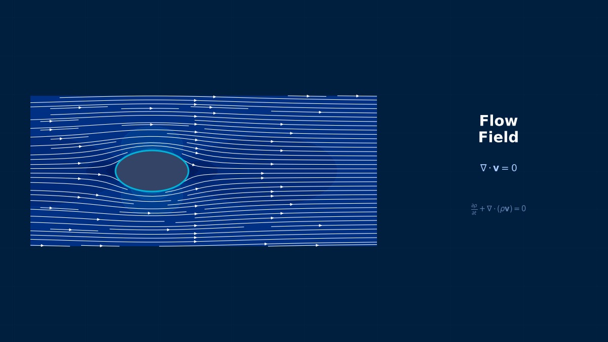
Overview
Professor, when is the energy equation for fluids necessary?
It is essential when you want to determine the temperature field. Designing heat exchangers, cooling electronic devices, combustion, natural convection—all require solving the energy equation. For isothermal flow, the NS equations and continuity equation alone form a closed system, but when temperature is involved, the energy equation is added.
Energy Equation (Temperature Form)
The energy equation for the temperature field in incompressible flow is as follows.
Here, $c_p$ is the specific heat at constant pressure, $k$ is the thermal conductivity, $\Phi$ is the viscous dissipation function, and $\dot{q}$ is the internal heat generation rate.
What is viscous dissipation?
It's the term where kinetic energy is converted to heat by viscosity. For incompressible flow,
In typical engineering flows, viscous dissipation is negligibly small, but it cannot be ignored for high-viscosity fluids (like polymer melts) or ultra-high-speed flows.
Eckert Number
The importance of viscous dissipation is evaluated by the Eckert number.
If $Ec \ll 1$, viscous dissipation is negligible. For example, in an air flow ($U = 50$ m/s, $\Delta T = 20$ K), $Ec \approx 0.12$, which is small. On the other hand, in polymer extrusion ($U = 0.1$ m/s, $\mu = 1000$ Pa·s), dissipation can be the main cause of temperature rise.
Energy Equation (Enthalpy Form)
How does it change for compressible flow?
The energy equation using total enthalpy $h_0 = h + \frac{1}{2}|\mathbf{u}|^2$ is used.
For compressible flow, the equation of state $p = \rho R T$ (ideal gas) is added, closing the system of equations. The four fields—density, velocity, pressure, and temperature—are all coupled.
Dimensionless Parameters
| Parameter | Definition | Physical Meaning |
|---|---|---|
| Prandtl Number Pr | $\nu/\alpha = \mu c_p/k$ | Ratio of momentum diffusivity to thermal diffusivity |
| Nusselt Number Nu | $hL/k$ | Ratio of convective to conductive heat transfer |
| Peclet Number Pe | $Re \cdot Pr$ | Ratio of advection to diffusion |
| Eckert Number Ec | $U^2/(c_p\Delta T)$ | Kinetic energy / Thermal energy |
So, while the Pr number is determined by the fluid properties, the Nu number is obtained as a calculation result, right?
Exactly. Air has $Pr \approx 0.71$, water has $Pr \approx 7$, and engine oil has $Pr \approx 100$–1000. A larger Pr number means a thinner thermal boundary layer, requiring finer meshes to accurately resolve the temperature gradient near the wall.
History of the Energy Equation—From Joule's Heat-Work Equivalence Experiment (1843) to Fluid Mechanics
The concept of the mechanical equivalent of heat included in the fluid energy equation was established by the British scientist James Joule in 1843 through his water stirring experiment. The Joule constant, 1 cal = 4.186 J, remains a fundamental constant in thermodynamics. Its integration into fluid mechanics came from combining Fourier's heat conduction equation (1822) with the Navier-Stokes equations, and the standard form of the energy equation was established in the 1850s. In particular, the "Viscous Dissipation" term—the effect where velocity gradients are converted to heat—cannot be ignored in supersonic or high-viscosity flows and is a term that must be enabled in modern CFD for high-accuracy analysis. While it is often omitted in low-speed, low-viscosity engineering CFD, it's important to recognize its applicability limit (Br=ηU²/(kΔT)>0.1).
Computational Methods for Energy Equation of Fluids
Discretization of the Energy Equation
How is the energy equation solved numerically?
In the finite volume method, the advection and diffusion terms are discretized as cell face fluxes.
A characteristic point is that the energy equation is a scalar transport equation and can be solved as a linear problem if the velocity field is known. An approach is possible where the energy equation is solved as a post-processing step after solving the NS equations.
Advection Scheme Selection
Is the advection scheme for the temperature field the same as for the velocity field?
When the Pe number (Peclet Number) is large, advection dominates, and central differencing causes numerical oscillations. Generally, as follows.
| Pe Number Range | Recommended Scheme | Remarks |
|---|---|---|
| Pe < 2 | Central Differencing (CD) | Stable for diffusion-dominated flows |
| Pe > 2 | Upwind Differencing (Upwind) | Has numerical diffusion |
| High Accuracy | QUICK, TVD (MUSCL, etc.) | Balances accuracy and stability |
Thermal Boundary Conditions
There are mainly three types of thermal boundary conditions at walls.
| Boundary Condition | Mathematical Expression | Applications |
|---|---|---|
| Fixed Temperature (1st Kind) | $T_{wall} = T_0$ | Cooling water wall, constant temperature bath |
| Fixed Heat Flux (2nd Kind) | $-k\frac{\partial T}{\partial n} = q_w$ | Heater, heat-generating surface |
| Convective Heat Transfer (3rd Kind) | $-k\frac{\partial T}{\partial n} = h(T - T_\infty)$ | Heat exchange with external environment |
Temperature Field in Turbulence
For turbulent flow, is a model also needed for the temperature field?
In RANS, modeling of the turbulent heat flux $\overline{u_i'T'}$ is required. The most common is the eddy diffusivity model.
$Pr_t$ (Turbulent Prandtl Number) is typically set to 0.85–0.9. The temperature profile near the wall (e.g., Jayatilleke's wall function) is also important.
How much does the turbulent Pr number affect the results?
It affects wall heat transfer rate by about 10–20%. Especially for liquid metals ($Pr \ll 1$, $Pr_t \approx 1$–4), the standard value of 0.85 is inaccurate. For liquid metals, dedicated models are necessary.
Discretization of the Energy Equation—"Implicit or Explicit?" is Determined by the Rate of Temperature Change
When solving the fluid energy equation numerically, the choice between explicit and implicit methods greatly affects computational efficiency. Explicit methods are simple to implement but are bound by the stability condition for heat diffusion Δt≤ρcΔx²/(2k). In models mixing insulation and metal, where thermal conductivity differs by a factor of 100, the stable Δt is constrained by the thinnest metal cell, causing the overall computation time to explode. Switching to an implicit method at this point allows Δt to be set much larger. "The equation form is the same," but changing the discretization strategy can change computation time by tens of times—this is the reality of numerical methods.
Experience the theory firsthand with the interactive simulator for this field
All Simulators