個数密度関数法(PBM)
Theory and Physics
Overview
Professor, what is the Population Balance Method (PBM)?
The PBM (Population Balance Model) is a model that tracks the spatiotemporal changes in the size distribution of bubbles, droplets, and particles. It describes the process by which the size distribution changes due to coalescence, breakup, nucleation, and growth.
In what situations is it used?
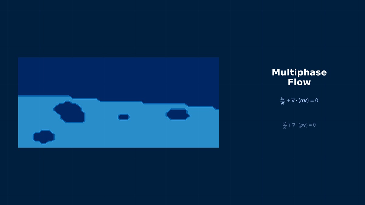
It is used in a wide range of problems where the size distribution of a dispersed phase is important, such as bubble size distribution in bubble columns, droplet size distribution in emulsification processes, crystal size distribution in crystallization, and particle size changes in aerosols. It is commonly used in combination with the Euler-Euler method.
Governing Equations
Please tell me the PBM equation.
The transport equation for the number density $n(V, \mathbf{x}, t)$ of particles (bubbles/droplets) with volume $V$ is as follows.
Each term on the right-hand side represents the following.
- $B_{coal}$: Generation by coalescence (two smaller particles coalesce to form size V)
- $D_{coal}$: Disappearance by coalescence (a particle of size V coalesces with another to become larger)
- $B_{break}$: Generation by breakup (a large particle breaks up to produce size V)
- $D_{break}$: Disappearance by breakup (a particle of size V breaks up into smaller ones)
How are the coalescence and breakup rates modeled?
Let me show you some representative closure models.
| Process | Model Example | Driving Mechanism |
|---|---|---|
| Coalescence Frequency | Prince & Blanch (1990) | Turbulent collision + film drainage |
| Coalescence Frequency | Luo (1993) | Turbulent energy |
| Breakup Frequency | Luo & Svendsen (1996) | Breakup by turbulent eddies |
| Breakup Frequency | Martínez-Bazán (2010) | Inertia-surface tension balance |
Sauter Mean Diameter
How do you obtain a representative diameter from the size distribution?
The Sauter mean diameter $d_{32}$ is most commonly used.
$m_k = \int_0^\infty V^{k/3} n(V) dV$ is the $k$-th moment of the distribution. $d_{32}$ corresponds to the volume-to-surface area ratio and is suitable for evaluating mass transfer and reaction rates.
Population Balance—Multiphase Flow Theory as Engineering's "Evolution Theory"
The Population Balance Equation (PBE) is a versatile framework for describing the spatiotemporal changes of populations possessing "internal coordinates" such as size, age, and composition. It is mathematically isomorphic to biological population dynamics (Lotka-Volterra equations) and can uniformly handle everything from bubble distributions and crystal size distributions to cell concentration distributions. The application of PBE in chemical engineering was pioneered by Randolph & Larson's 1971 paper on crystallization, and 50 years later, it has evolved into a design tool for pharmaceutical manufacturing, bubble columns, and liquid-liquid extraction as C-PBE (Coupled PBE) coupled with CFD.
Physical Meaning of Each Term
- Time Term $\partial(\rho\phi)/\partial t$: Imagine the moment you turn on a faucet. At first, water comes out in an unstable, spluttering manner, but after a while, the flow becomes steady, right? This "period of change" is described by the time term. The pulsation of blood flow due to the heartbeat, and the flow fluctuation each time an engine valve opens and closes are all unsteady phenomena. So what is steady-state analysis? It looks only at "after sufficient time has passed and the flow has settled down"—in other words, setting this term to zero. Since this significantly reduces computational cost, solving first in steady-state is a basic CFD strategy.
- Convection Term $\nabla \cdot (\rho \mathbf{u} \phi)$: What happens if you drop a leaf into a river? It gets carried downstream by the flow, right? This is "convection"—the effect where fluid motion transports things. Warm air from a heater reaching the far end of a room is also because the "carrier," air, transports heat via convection. Here's the interesting part—this term contains "velocity × velocity," making it nonlinear. That is, as the flow becomes faster, this term rapidly strengthens, making control difficult. This is the root cause of turbulence. A common misconception: "Convection and conduction are similar things" → They are completely different! Convection is carried by flow, conduction is transmitted by molecules. There is an order of magnitude difference in efficiency.
- Diffusion Term $\nabla \cdot (\Gamma \nabla \phi)$: Have you ever put milk in coffee and left it? Even without stirring, after a while, it naturally mixes, right? That's molecular diffusion. Now, next question—honey and water, which flows more easily? Obviously water, right? Honey has high viscosity ($\mu$), so it flows poorly. When viscosity is high, the diffusion term becomes strong, and the fluid moves in a "sluggish" manner. In low Reynolds number flows (slow, viscous), diffusion is dominant. Conversely, in high Re number flows, convection overwhelms, and diffusion becomes a supporting role.
- Pressure Term $-\nabla p$: When you push the plunger of a syringe, liquid comes out forcefully from the needle tip, right? Why? Because the piston side is high pressure, the needle tip is low pressure—this pressure difference becomes the force that pushes the fluid. Dam discharge works on the same principle. On a weather map, where isobars are densely packed? That's right, strong winds blow. "Where there is a pressure difference, flow is generated"—this is the physical meaning of the pressure term in the Navier-Stokes equations. A point of confusion here: "Pressure" in CFD is often gauge pressure, not absolute pressure. When you switch to compressible analysis and suddenly get strange results, it might be due to confusion between absolute/gauge pressure.
- Source Term $S_\phi$: Heated air rises—why? Because it becomes lighter (lower density) than its surroundings, so it is pushed up by buoyancy. This buoyancy is added to the equation as a source term. Other examples: chemical reaction heat generated by a gas stove flame, Lorentz force acting on molten metal in a factory's electromagnetic pump... These are all actions that "inject energy or force into the fluid from the outside" and are expressed by source terms. What happens if you forget the source term? In natural convection analysis, if you forget to include buoyancy, the fluid doesn't move at all—a physically impossible result where warm air doesn't rise in a room with the heater on in winter.
Assumptions and Applicability Limits
- Continuum assumption: Valid for Knudsen number Kn < 0.01 (mean free path ≪ characteristic length)
- Newtonian fluid assumption: Linear relationship between shear stress and strain rate (viscosity model needed for non-Newtonian fluids)
- Incompressibility assumption (for Ma < 0.3): Treat density as constant. For Mach number ≥ 0.3, consider compressibility effects
- Boussinesq approximation (natural convection): Consider density changes only in the buoyancy term, use constant density in other terms
- Non-applicable cases: Rarefied gas (Kn > 0.1), supersonic/hypersonic flow (shock capturing required), free surface flow (VOF/Level Set etc. required)
Dimensional Analysis and Unit Systems
| Variable | SI Unit | Notes / Conversion Memo |
|---|---|---|
| Velocity $u$ | m/s | When converting from volumetric flow rate for inlet conditions, pay attention to cross-sectional area units |
| Pressure $p$ | Pa | Distinguish between gauge and absolute pressure. Use absolute pressure for compressible analysis |
| Density $\rho$ | kg/m³ | Air: approx. 1.225 kg/m³ @20°C, Water: approx. 998 kg/m³ @20°C |
| Viscosity coefficient $\mu$ | Pa·s | Be careful not to confuse with kinematic viscosity coefficient $\nu = \mu/\rho$ [m²/s] |
| Reynolds number $Re$ | Dimensionless | $Re = \rho u L / \mu$. Criterion for laminar/turbulent transition |
| CFL number | Dimensionless | $CFL = u \Delta t / \Delta x$. Directly related to time step stability |
Numerical Methods and Implementation
Details of Numerical Methods
Please tell me how to solve the PBM numerically.
The PBE is an integro-differential equation with volume (size) as an additional independent variable, making it difficult to solve directly. The following discretization methods are used.
| Method | Overview | Computational Cost | Accuracy |
|---|---|---|---|
| MUSIG (Multi-Size Group) | Divides size space into bins | High (proportional to number of bins) | Depends on bin count |
| QMOM (Quadrature MOM) | Method of Moments + quadrature formula | Low (6-8 moments) | Good |
| DQMOM | Direct Quadrature Method of Moments | Low | Good |
| S-Gamma | Two-parameter distribution assumption | Lowest | Constrained by distribution shape |
Please explain the difference between MUSIG and QMOM.
MUSIG divides the size space into 10-30 bins (size groups) and solves a transport equation for the number density in each bin. It is accurate, but since it solves additional transport equations equal to the number of bins, the computational cost is high.
QMOM (McGraw, 1997) does not directly solve for the size distribution, but solves transport equations for the first few moments ($m_0, m_1, ..., m_5$, etc.). It determines the nodes and weights of the quadrature formula using the Product-Difference Algorithm (PDA) or Wheeler's method to calculate the source terms for coalescence and breakup.
Implementation in Fluent
Implementation in STAR-CCM+
In STAR-CCM+, the S-Gamma model (Lo, 2000) is standard, tracking the distribution with two parameters (mean diameter and variance). It has the lowest computational cost, but the distribution shape is constrained to a gamma distribution. MUSIG is also available.
Implementation in OpenFOAM
In OpenFOAM, the populationBalanceModel class has been available since v2006. MUSIG (including iMUSIG) and QMOM are implemented. Configuration is done in populationBalanceCoeffs within constant/phaseProperties.
QMOM vs DQMOM—Trade-offs in the Method of Moments
The Method of Moments is used to realistically control the computational cost of CFD-PBE. QMOM (Quadrature Method of Moments) approximates the distribution function at quadrature points and solves only the moment equations to track the temporal evolution of the entire distribution. However, in systems with complex breakup/coalescence, the "moment inversion problem" occurs where quadrature points intersect. DQMOM (Direct QMOM) avoids this problem by directly solving transport equations for the position and weight of each quadrature point, but the nonlinearity of the source terms makes convergence difficult. In CFD benchmarks for bubble columns, there are many cases where QMOM and DQMOM predictions for bubble size distribution differ by 10-20%, indicating that model selection has a non-negligible impact on results.
Upwind Scheme (Upwind)
First-order upwind: Large numerical diffusion but stable. Second-order upwind: Improved accuracy but risk of oscillations. Essential for high Reynolds number flows.
Central Differencing (Central Differencing)
Second-order accurate, but numerical oscillations occur for Pe number > 2. Suitable for low Reynolds number diffusion-dominated flows.
TVD Scheme (MUSCL, QUICK, etc.)
Suppresses numerical oscillations while maintaining high accuracy using limiter functions. Effective for capturing shock waves and steep gradients.
Finite Volume Method vs Finite Element Method
FVM: Naturally satisfies conservation laws. Mainstream in CFD. FEM: Advantageous for complex shapes and multiphysics. Mesh-free methods like SPH are also developing.
CFL Condition (Courant Number)
Explicit method: CFL ≤ 1 is the stability condition. Implicit method: Stable even for CFL > 1, but affects accuracy and iteration count. LES: CFL ≈ 1 recommended. Physical meaning: Information should not travel more than one cell per timestep.
Residual Monitoring
Convergence is judged when residuals for continuity, momentum, and energy decrease by 3-4 orders of magnitude. The mass conservation residual is particularly important.
Relaxation Factor
Typical initial values: Pressure: 0.2-0.3, Velocity: 0.5-0.7. If diverging, lower the relaxation factor. After convergence, increase to accelerate.
Internal Iterations for Unsteady Calculations
Iterate within each timestep until a steady solution converges. Internal iteration count: 5-20 times is a guideline. If residuals fluctuate between timesteps, review the timestep size.
Analogy for the SIMPLE Method
The SIMPLE method is an "alternating adjustment" technique. First, velocity is tentatively determined (predictor step), then pressure is corrected so that mass conservation is satisfied with that velocity (corrector step), and velocity is revised using the corrected pressure—this back-and-forth is repeated to approach the correct solution. It resembles two people leveling a shelf: one adjusts the height, the other balances it, and they repeat this alternately.
Analogy for the Upwind Scheme
The upwind scheme is a method that "stands in the river flow and prioritizes upstream information." A person in the river cannot tell the source of the water by looking downstream—it reflects the physics that upstream information determines downstream, making it a discretization method. It is first-order accurate but highly stable because it correctly captures flow direction.
Practical Guide
Practical Guide
Please tell me the procedure for PBM analysis.
Let me explain using bubble size distribution analysis in a bubble column as an example.
Related Topics
なった
詳しく
報告