Solidification and Casting Simulation
Solidification and Casting: Theoretical Foundations
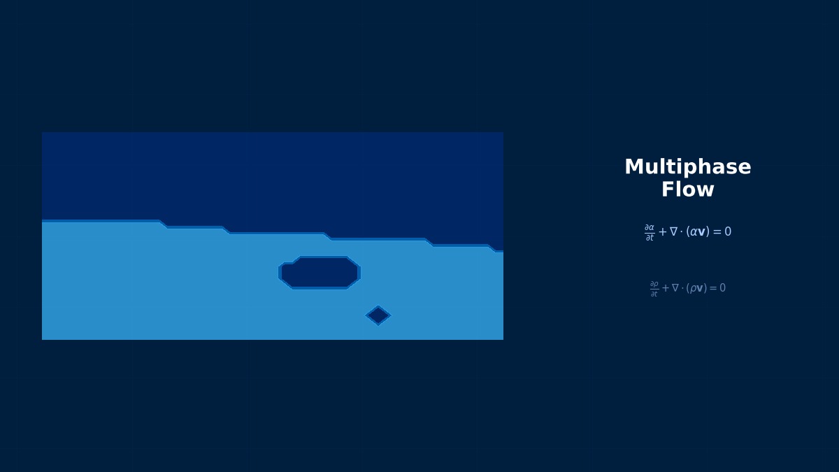
Overview
Professor, what does CFD for solidification calculate?
It predicts the process where molten metal cools and solidifies. It deals with flow and heat transfer problems involving solid-liquid phase changes, such as mold filling and solidification analysis in casting, shell growth in continuous casting, bead formation in welding, and molten pool behavior in metal 3D printing (PBF/DED).
You handle liquid turning into solid using fluid dynamics?
The Enthalpy Method (Enthalpy-Porosity method) is the standard approach. It does not explicitly track the solid-liquid interface; instead, it represents the progress of solidification using the liquid fraction $f_L$ (a continuous variable from 0 to 1) in each cell.
Governing Equations
Please tell me the equations for the Enthalpy Method.
The energy equation is described in terms of enthalpy $H$.
Enthalpy is the sum of sensible heat and latent heat.
$h = \int_{T_{ref}}^{T} c_p dT$ is the sensible heat, $f_L$ is the liquid fraction, and $L$ is the latent heat of solidification. The liquid fraction is determined from the liquidus temperature $T_L$ and solidus temperature $T_S$.
What happens to the flow in the solidified part?
In the Enthalpy-Porosity method, the solidified region is treated as a porous medium with high resistance. A Darcy drag source term is added to the momentum equation.
$C$ is the Mushy zone constant (typical values $10^5$ to $10^8$), $\epsilon$ is a small constant to avoid division by zero, and $\mathbf{u}_{pull}$ is the pulling speed (in continuous casting). As $f_L \to 0$ (complete solidification), the source term approaches infinity, causing the velocity to decay to zero.
Marangoni Convection
What are the driving forces for flow in a molten pool?
Marangoni convection, caused by the temperature dependence of surface tension ($d\sigma/dT$), dominates the flow pattern in the molten pool.
For many metals, $d\sigma/dT < 0$ (surface tension is lower at higher temperatures), causing an outward flow from the center of the molten pool. However, the sign can reverse depending on oxygen or sulfur content, dramatically changing the flow pattern.
The Microscopic World of Solidification—Dendrite Growth and the Stefan Problem
The physics of metal solidification is formulated as a Stefan problem: "How does the solid-liquid interface move?" For pure metals, the interface moves along the melting point isotherm, and its speed is determined by the balance between latent heat and heat flux. However, in actual alloys, constitutional supercooling occurs locally, leading to the spontaneous formation of complex dendritic solid-liquid interfaces. The Phase-Field method, which directly calculates this dendrite growth in CFD, has rapidly developed since the 1990s, and by the 2020s, dendrite calculations with 10^6 meshes became possible on GPUs at speeds close to real-time.
Computational Methods for Solidification and Casting
Details of Numerical Methods
Please tell me the numerical points for solidification simulation.
The biggest challenge is handling the latent heat of solidification. The release of latent heat creates nonlinearity in enthalpy and causes abrupt changes in the temperature field. Time step management and convergence of iterative calculations are key.
Influence of Mushy Zone Constant
How do you set the Mushy zone constant $C$?
The value of $C$ has a significant impact on the results.
| Value of $C$ | Effect | Application |
|---|---|---|
| $10^4$ to $10^5$ | Gentle damping | Slow solidification, continuous casting |
| $10^5$ to $10^6$ | Standard | General casting |
| $10^7$ to $10^8$ | Rapid damping | Rapid solidification, welding |
Ideally, it should be determined from experimental data on Darcy permeability, but in practice, it's common to start with $10^5$ to $10^6$ and perform a sensitivity analysis.
Coupling with VOF Method
How is the mold filling process in casting calculated?
The filling process tracks the free surface of the molten metal using the VOF method, and solidification is calculated after filling is complete (or simultaneously with filling). In Fluent or Flow-3D, simultaneous calculation with VOF + Solidification/Melting models is possible.
Flow patterns during filling, oxide film entrapment, and gas entrainment directly lead to casting defects, making filling analysis a crucial element of casting simulation.
Implementation by Tool
| Tool | Solidification Model | VOF Coupling | Stress Analysis Linkage |
|---|---|---|---|
| Ansys Fluent | Solidification/Melting | Supported | Mechanical Integration |
| Flow-3D | TruVOF + Solidification | Native | Limited |
| STAR-CCM+ | Solidification | Supported | Structural Coupling |
| ProCAST (ESI) | FEM Solidification + Filling | Dedicated Filling | Integrated Stress/Deformation Analysis |
| MAGMASOFT | Proprietary FVM | Proprietary Model | Residual Stress Prediction |
ProCAST and MAGMASOFT are dedicated casting software, right?
That's correct. They are specialized tools dedicated to casting processes, capable of integrated calculation of filling, solidification, shrinkage prediction, and deformation. They are more equipped with casting-specific physics models (e.g., feeding, Niyama criterion) than general-purpose CFD.
Enthalpy-Porosity Method—The Standard Approach for Practical Solidification CFD
The most widely used method in industrial solidification CFD (continuous casting, mold filling) is the Enthalpy-Porosity method. It treats the solid-liquid coexistence region (mushy zone) as a "porous medium with low permeability" and reproduces the progress of solidification by suppressing local velocity using the Kozeny-Carman equation. This approach was proposed by Voller & Prakkash in 1987 and is implemented in ANSYS Fluent's solidificationMeltingSource and OpenFOAM. The model characterization constant (Amush) often uses a default value of 1.6x10^5, but if this value is inappropriate, the solidification speed can deviate by 30-50%.