Nonlinear Analysis of Cables and Ropes
Nonlinear Analysis of Cables and Ropes: Theoretical Foundations
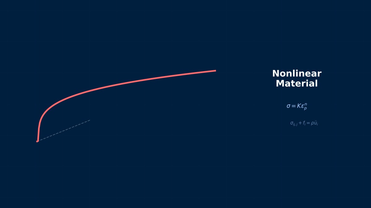
Cable Nonlinearity
Professor, why is cable analysis nonlinear?
Cables have zero compressive stiffness (only transmit tension) and their shape changes significantly under load. Like a catenary (suspended cable), they sag under self-weight, and their stiffness changes with tension. They are inherently geometrically nonlinear.
Catenary Theory
Catenary curve of a cable under self-weight:
$H$ is horizontal tension, $w$ is weight per unit length.
Modeling in FEM
- Truss element (tension only) — Zero compressive stiffness. NLGEOM=YES is mandatory.
- Beam element (with bending) — For wire ropes. Bending stiffness is small but non-zero.
- Abaqus *NO COMPRESSION — Element deactivates under compression.
Summary
- Cables are inherently geometrically nonlinear — Stiffness changes with tension.
- NLGEOM=YES is mandatory — Linear analysis is meaningless.
- Truss element (tension only) or Beam element — Choose based on presence of bending.
Suspension Bridge Cables and the Chain Problem
The natural shape (catenary curve) of a suspension bridge cable was mistakenly described as a parabola by Galileo in 1638, and the correct formula y=a·cosh(x/a) was derived by Huygens in 1691. The equation for this catenary curve was also solved independently around the same time by Leibniz and Bernoulli, making it one of the most intense examples of independent discovery competition in mathematical history. FEM cable analysis finds the suspended shape through geometrically nonlinear iterations that update nodal coordinates.
Computational Methods for Nonlinear Analysis of Cables and Ropes
FEM Settings for Cables
```
*ELEMENT, TYPE=T3D2 $ 3D truss element
*NO COMPRESSION $ No compression
*STEP, NLGEOM=YES
*STATIC
```
Determining Initial Shape (Form-finding)
Finding the initial shape (catenary) of a cable using FEM:
1. Apply self-weight to the cable.
2. Find the equilibrium shape with NLGEOM=YES.
3. Use the obtained shape as the initial shape.
Summary
- Truss element + NO COMPRESSION + NLGEOM=YES
- Determine initial shape via shape analysis (form-finding)
Cable Finite Element Formulation and Elastic Catenary
FEM for cables includes bar elements (tension only) and more accurate elastic catenary elements. Elastic catenary elements analytically account for self-weight and elastic deformation within the element, allowing accurate shape representation even for long cables (spanning hundreds of meters) with just a few elements. To achieve the same accuracy with bar elements, mesh refinement is needed so that sag per element is less than 2% of the slack, increasing the number of elements by 50-100 times.
Nonlinear Analysis of Cables and Ropes in Practice
Cable Practical Work
Suspension bridge cables, power transmission lines, marine risers, crane wires, etc.
Practical Checklist
- [ ] Is NLGEOM=YES set?
- [ ] Is zero compressive stiffness configured?
- [ ] Are initial tension/initial shape correct (catenary)?
- [ ] Are self-weight and additional loads (wind, ice, etc.) included?
- [ ] Does cable sag match theoretical values?
Akashi Kaikyō Bridge Cable Analysis
The main cables of the Akashi Kaikyō Bridge (main span 1991m, completed 1998) consist of 290 bundles of Φ127mm PWS (Parallel Wire Strand), with a single cable diameter of 1.12m and total weight of 50,000 tons. During design, shape changes due to wind loads, earthquakes, and temperature variations were evaluated using FEM nonlinear cable analysis, confirming that the deflection at the top of the main towers would be up to 3.8m (for a design temperature difference of 50°C).
Nonlinear Analysis of Cables and Ropes: Software & Solver Comparison
Cable Tools
- General-purpose FEM — Truss/beam elements + NLGEOM
- OrcaFlex — Dedicated for marine structure cables/risers
- SAP2000 — For suspension bridge cable analysis
- PLS-CADD — For power transmission line design
SAP2000 Cable Element Track Record
Computers & Structures' SAP2000 is a standard software for cable structure analysis, featuring a standard elastic catenary cable element. It is used worldwide for designing cable-stayed bridges, suspension bridges, and tensegrity structures, and was also used for the nonlinear analysis of the dome stadium in Kaohsiung, Taiwan (300m diameter cable roof). Its OAPI (Open Application Programming Interface), which allows automation of analysis from Python, is highly valued by design firms.
Advanced Technology
Advanced Cable Research
- Wind-cable coupling — Simulation of vortex-induced vibration (galloping).
- Tension monitoring — Non-destructive estimation of cable tension from vibration frequency.
Wind-induced Vibration and Cable Dynamic Instability
Cables of long-span bridges face problems with "rain-wind induced vibration". When raindrops adhere to the cable surface, changing its cross-sectional shape, aerodynamic instability (galloping) can be induced. This phenomenon, which occurred on the Yokohama Bay Bridge in the 1990s, was addressed by installing dampers (vibration control devices) and applying surface grooving. The phenomenon was reproduced and analyzed through coupled simulation of FFT analysis and elastic cable FEM.
Nonlinear Analysis of Cables and Ropes: Common Issues & Debugging
Cable Troubles
Common issues:
- Convergence failure — NLGEOM=YES not set, or initial tension too low.
- Unphysical cable shapes — Check boundary conditions and element orientation.
- Snap-through buckling — Use arc-length control for snap-through phenomena.