連続体損傷力学(CDM)

Category: 構造解析 | Integrated 2026-04-06
CAE visualization for damage continuum theory - technical simulation diagram
連続体損傷力学(CDM)

Theory and Physics

What is CDM?

🧑‍🎓

Professor, what is Continuum Damage Mechanics (CDM)?


🎓

CDM (Continuum Damage Mechanics) is a theory that describes material degradation (damage) using a continuous variable $D$. Proposed by Kachanov (1958) and Rabotnov (1968).


$$ \tilde{\sigma} = \frac{\sigma}{1-D} $$

$D = 0$ for intact material, $D = 1$ for complete failure. $\tilde{\sigma}$ is the effective stress.


CDM Framework

🎓

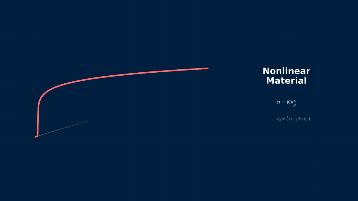
Stress-strain relation:

$$ \sigma = (1-D) C \varepsilon $$

Damage evolution law (example: creep damage):

$$ \dot{D} = A \left(\frac{\sigma}{1-D}\right)^n $$

🧑‍🎓

As damage progresses, the effective stress increases, leading to further acceleration of damage—a positive feedback loop.


🎓

This "chain reaction" leads to final failure ($D \to 1$). CDM provides a unified framework for creep fracture, fatigue, and ductile fracture.


Summary

🎓
  • Damage variable $D$ (0~1) describes material degradation — within a continuum framework
  • Effective stress $\tilde{\sigma} = \sigma/(1-D)$ — effective stress increases with damage
  • Creep damage, fatigue damage, ductile damage — applications of CDM
  • Hashin damage (composites) is also a type of CDM

  • Coffee Break Yomoyama Talk

    Kachanov's 1958 Paper

    The foundation of Continuum Damage Mechanics (CDM) lies in a mere 8-page Russian paper "On the Creep Fracture Time" published by L.M. Kachanov in 1958. He introduced the concept of "effective stress" and represented the accumulation of microcracks with a single scalar damage variable ω. Although Kachanov was marginalized in the Soviet Union at the time, after being introduced to the West in the 1980s, his work rapidly gained attention and led to the systematization of CDM by Lemaitre and Chaboche.

    Physical Meaning of Each Term
    • Inertia term (mass term): $\rho \ddot{u}$, i.e., "mass × acceleration". Have you ever experienced being thrown forward when slamming on the brakes? That "feeling of being carried forward" is precisely the inertial force. Heavier objects are harder to set in motion and harder to stop once moving. Buildings shake during earthquakes because the ground moves suddenly while the building's mass "gets left behind". In static analysis, this term is set to zero, which assumes "forces are applied slowly enough that acceleration can be ignored". It absolutely cannot be omitted for impact loads or vibration problems.
    • Stiffness term (elastic restoring force): $Ku$ or $\nabla \cdot \sigma$. When you stretch a spring, you feel a "force trying to return it", right? That's Hooke's law $F=kx$, the essence of the stiffness term. Now a question—if you pull an iron rod and a rubber band with the same force, which stretches more? Obviously the rubber band. This "resistance to stretching" is the Young's modulus $E$, which determines stiffness. A common misconception: "High stiffness = strong" is incorrect. Stiffness is "resistance to deformation", strength is "resistance to failure"—they are different concepts.
    • External force term (load term): Body forces $f_b$ (gravity, etc.) and surface forces $f_s$ (pressure, contact forces, etc.). Think of it this way—the weight of a truck on a bridge is a "force acting on the entire volume" (body force), while the force of the tires pushing on the road surface is a "force acting only on the surface" (surface force). Wind pressure, water pressure, bolt tightening force... all are external forces. A common pitfall here: getting the load direction wrong. Intending "tension" but modeling "compression"—it sounds like a joke, but it actually happens when coordinate systems are rotated in 3D space.
    • Damping term: Rayleigh damping $C\dot{u} = (\alpha M + \beta K)\dot{u}$. Try plucking a guitar string. Does the sound continue forever? No, it gradually fades away. That's because vibrational energy is converted to heat through air resistance and internal friction in the string. Car shock absorbers work on the same principle—they intentionally absorb vibrational energy to improve ride comfort. What if damping were zero? Buildings would keep swaying forever after an earthquake. Since that doesn't happen in reality, setting appropriate damping is crucial.
    Assumptions and Applicability Limits
    • Continuum assumption: Treats material as a continuous medium, ignoring microscopic inhomogeneities.
    • Small deformation assumption (for linear analysis): Deformation is sufficiently small compared to initial dimensions, and the stress-strain relationship is linear.
    • Isotropic material (unless otherwise specified): Material properties are independent of direction (anisotropic materials require separate tensor definitions).
    • Quasi-static assumption (for static analysis): Ignores inertial and damping forces, considering only the balance between external and internal forces.
    • Non-applicable cases: For large deformation/large rotation problems, geometric nonlinearity is required. For nonlinear material behavior like plasticity and creep, constitutive law extensions are needed.
    Dimensional Analysis and Unit Systems
    VariableSI UnitNotes / Conversion Memo
    Displacement $u$m (meter)When inputting in mm, unify loads and elastic modulus to MPa/N system.
    Stress $\sigma$Pa (Pascal) = N/m²MPa = 10⁶ Pa. Be careful of unit system inconsistency when comparing with yield stress.
    Strain $\varepsilon$Dimensionless (m/m)Note the distinction between engineering strain and logarithmic strain (for large deformations).
    Elastic modulus $E$PaSteel: ~210 GPa, Aluminum: ~70 GPa. Note temperature dependence.
    Density $\rho$kg/m³In mm system: tonne/mm³ (= 10⁻⁹ tonne/mm³ for steel).
    Force $F$N (Newton)Unify as N in mm system, N in m system.

    Numerical Methods and Implementation

    CDM in FEM

    🎓

    Abaqus's composite Hashin damage and Ductile Damage are CDM-based. Custom CDM models can be implemented via user subroutines (UMAT/VUMAT).


    Summary

    🎓
    • Abaqus's *DAMAGE family is CDM-based — Hashin, Ductile, Shear, etc.
    • Custom CDM via UMAT/VUMAT — arbitrary damage evolution laws
    • Regularization via fracture energy — eliminates mesh dependency

    • Coffee Break Yomoyama Talk

      Lemaitre's Damage-Plasticity Coupling Model

      Jean Lemaitre, born in Chambon, France, extended Kachanov's uniaxial theory to three-dimensional elastoplastic damage mechanics in his 1984 paper "How to Use Damage Mechanics". Damage is defined as an isotropic scalar D, and by replacing stress with effective stress σ̃ = σ/(1−D), it can be easily coupled with existing plasticity models. The Lemaitre model is now included in the standard material libraries of France's Code_Aster and SYSTUS (by ESI).

      Linear Elements (1st-order elements)

      Linear interpolation between nodes. Low computational cost but low stress accuracy. Beware of shear locking (mitigated with reduced integration or B-bar method).

      Quadratic Elements (with mid-side nodes)

      Can represent curved deformation. Stress accuracy improves significantly, but degrees of freedom increase by about 2-3 times. Recommended when stress evaluation is important.

      Full integration vs Reduced integration

      Full integration: Risk of over-constraint (locking). Reduced integration: Risk of hourglass modes (zero-energy modes). Choose appropriately for the situation.

      Adaptive Mesh

      Automatic refinement based on error indicators (e.g., ZZ estimator). Efficiently improves accuracy in stress concentration areas. Includes h-method (element subdivision) and p-method (order increase).

      Newton-Raphson Method

      Standard method for nonlinear analysis. Updates the tangent stiffness matrix every iteration. Achieves quadratic convergence within the convergence radius, but computational cost is high.

      Modified Newton-Raphson Method

      Updates the tangent stiffness matrix using the initial value or every few iterations. Cost per iteration is low, but convergence speed is linear.

      Convergence Criteria

      Force residual norm: $||R|| / ||F_{ext}|| < \epsilon$ (typically $\epsilon = 10^{-3}$ to $10^{-6}$). Displacement increment norm: $||\Delta u|| / ||u|| < \epsilon$. Energy norm: $\Delta u \cdot R < \epsilon$

      Load Increment Method

      Instead of applying the full load at once, it is applied in small increments. The arc-length method (Riks method) can trace beyond limit points on the load-displacement curve.

      Analogy: Direct Method vs Iterative Method

      The direct method is like "solving simultaneous equations accurately with pen and paper"—reliable but takes too long for large-scale problems. The iterative method is like "repeatedly guessing to approach the correct answer"—starts with a rough answer but improves accuracy with each iteration. It's the same principle as looking up a word in a dictionary: it's more efficient to estimate where to open it and adjust forward/backward (iterative method) than to search sequentially from the first page (direct method).

      Relationship Between Mesh Order and Accuracy

      1st-order elements are like "approximating a curve with a ruler"—represented by straight line segments, so accuracy is limited. 2nd-order elements are like "flexible curves"—can represent curved changes, dramatically improving accuracy even at the same mesh density. However, computational cost per element increases, so judge based on total cost-effectiveness.

      Practical Guide

      CDM in Practice

      🎓

      Used for metal ductile fracture (damage index), progressive damage in composites, and damage plasticity in concrete.


      Practical Checklist

      🎓
      • [ ] Is the damage initiation criterion based on material tests?
      • [ ] Is damage evolution regularized by fracture energy?
      • [ ] Is element deletion set for elements where damage variable $D$ reaches 1.0?
      • [ ] Has mesh convergence been verified? (Damage tends to localize)

      • Coffee Break Yomoyama Talk

        Application to Automotive Crash Analysis

        CDM also plays an important role in automotive crash safety (crash) analysis. Since the early 2000s, Volkswagen has adopted a combination of LS-DYNA's Gurson-Tvergaard-Needleman (GTN) model and CDM for sheet metal fracture prediction, utilizing it in occupant protection performance evaluation for frontal crash tests (Euro NCAP). It is reported that introducing CDM enabled predicting perforation fracture of high-strength steel (780 MPa grade) with 30% higher accuracy compared to the conventional maximum strain criterion.

        Analogy of Analysis Flow

        The analysis flow is actually very similar to cooking. First, you buy ingredients (prepare the CAD model), do the prep work (mesh generation), apply heat (solver execution), and finally plate it (visualization in post-processing). Here's an important question—which step in cooking is most prone to failure? Actually, it's the "prep work". If mesh quality is poor, the results will be a mess no matter how excellent the solver is.

        Pitfalls Beginners Often Fall Into

        Are you checking mesh convergence? Do you think "the calculation ran = the result is correct"? This is actually the most common trap for CAE beginners. The solver will always return "some answer" for the given mesh. But if the mesh is too coarse, that answer can be far from reality. Verify that results stabilize across at least three levels of mesh density—neglecting this leads to the dangerous assumption that "the computer gave the answer, so it must be correct".

        Thinking About Boundary Conditions

        Setting boundary conditions is like "writing the problem statement" for an exam. If the problem statement is wrong? No matter how accurately you calculate, the answer will be wrong. "Is this surface really fully fixed?" "Is this load really uniformly distributed?"—Correctly modeling real-world constraints is often the most critical step in the entire analysis.

        Software Comparison

        CDM Tools

        🎓
        • Abaqus — *DAMAGE family (Hashin, Ductile, Shear, FLD). Most extensive.
        • LS-DYNA — *MAT_ADD_EROSION. Johnson-Cook fracture, etc.
        • UMAT/VUMAT — Custom CDM

        • Coffee Break Yomoyama Talk

          Implementation History of SIMULIA Damage Mechanics

          CDM was first standardly implemented in Abaqus in version 6.2 (2001), with a simplified version of the Lemaitre model implemented as "Ductile Damage". Subsequently, a Gurson-type void model was added in 6.14 (2014), and rebranding progressed as Abaqus 2019 from 2019, also adding a sheet metal fracture model coupled with FLD (Forming Limit Diagram). In the current Abaqus 2024, five types of ductile damage criteria and three types of shear damage criteria are available for selection.

          Three Most Important Questions for Selection

          • "What are you solving?": Does the required physical model/element type for Continuum Damage Mechanics (CDM) have support? For example, in fluids, the presence of LES support, and in structures, the ability to handle contact/large deformation make a difference.
          • "Who will use it?": For beginner teams, tools with rich GUIs are suitable; for experienced users, flexible script-driven tools are better. Similar to the difference between automatic transmission (GUI) and manual transmission (script) in cars.
          • "How far will it be extended?": Selection considering future expansion of analysis scale (HPC support), deployment to other departments, and integration with other tools leads to long-term cost reduction.

          Advanced Technologies

          Advanced CDM

          🎓
          • Phase-Field Method — Tracks damage as a continuous field. A natural extension of CDM.
          • Non-local CDM — Fundamental solution to mesh dependency.
          • Multi-scale CDM — Micro-scale damage (voids, cracks) → Macro-scale damage variable.

          • Coffee Break Yomoyama Talk

            Non-localization Theory and Eliminating Mesh Dependency

            Since CDM involves strain localization, standard local theory shows a pathological dependency where fracture energy approaches zero as mesh size becomes finer. In 1987, Bažant and Pijaudier-Cabot proposed "non-local damage mechanics", evaluating the damage variable as a weighted average of surrounding elements (influence radius l ≈ 3× maximum aggregate size) to eliminate this dependency. This method has been implemented as an extension in diaFEA and the latest Abaqus 2024.

            Troubleshooting

            CDM Troubles

            🎓
            • Mesh dependency → Regularize with fracture energy. Consider non-local CDM.
            • Related Topics

              関連シミュレーター

              この分野のインタラクティブシミュレーターで理論を体感しよう

              シミュレーター一覧
              この記事の評価
              ご回答ありがとうございます!
              参考に
              なった
              もっと
              詳しく
              誤りを
              報告
              参考になった
              0
              もっと詳しく
              0
              誤りを報告
              0
              Written by NovaSolver Contributors
              Anonymous Engineers & AI — サイトマップ